
Use Processing Templates to Derive Land Surface Temperature
Ever wondered how your neighborhood stacks up against others in your community regarding the urban heat island effect? In this three-blog series, you will learn about climate resilience indices. The series walks you through the steps to use a global collection of ready-to-use geographic information to derive input variables needed to calculate a heat resilience index (HRI). The resulting intervention-focused map can be used by local communities to prioritize census tracts for tree planting as one mitigation against urban heat islands.
Climate change impacts us all, and robust science says things will only worsen if we don’t act swiftly. According to NOAA, scientists say that by the year 2100, average global temperatures will increase by 2 to 9.7°F (1.1 to 5.4°C).
Add Data from Living Atlas of the World
Let’s begin with a new ArcGIS Pro project. The first variable for the HRI is land surface temperature in degrees Celsius. You will derive this from the Multispectral Landsat imagery service in ArcGIS Living Atlas of the World. Using the Add Data button, search the Living Atlas for “Multispectral Landsat” and add it to the project. Be sure Living Atlas is selected under Portal on the left before typing your search text.
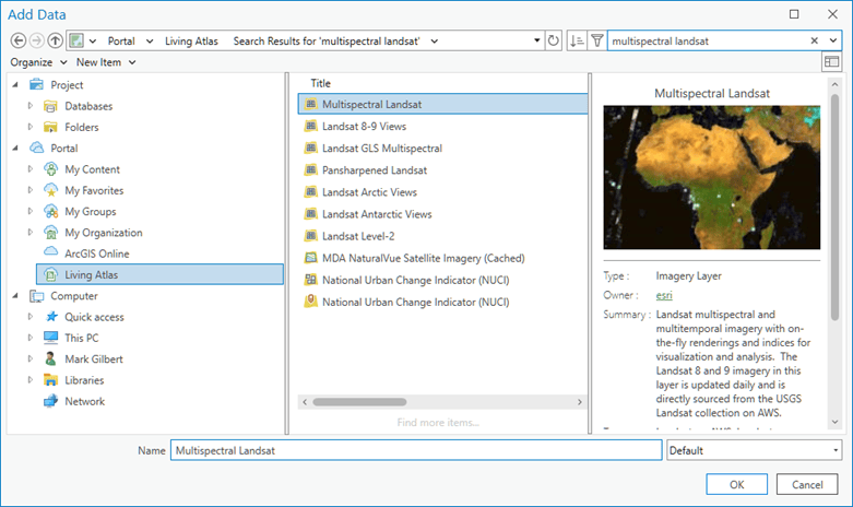
The Multispectral Landsat service contains decades’ worth of data, called scenes. The next few steps demonstrate how to use filtering and summarization tools to refine the data.
Change the Image Service Properties
You need to adjust the Landsat service properties to get the temperature data. Right-click the Multispectral Landsat service in Contents and select Properties.
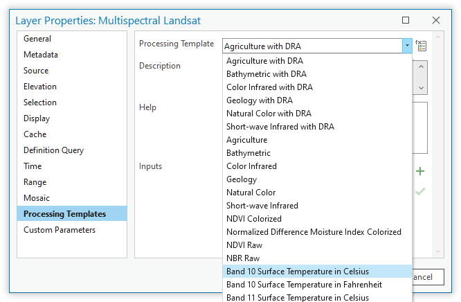
Select Processing Templates and choose “Band 10 Surface Temperature in Celsius” from the Processing Template drop-down.
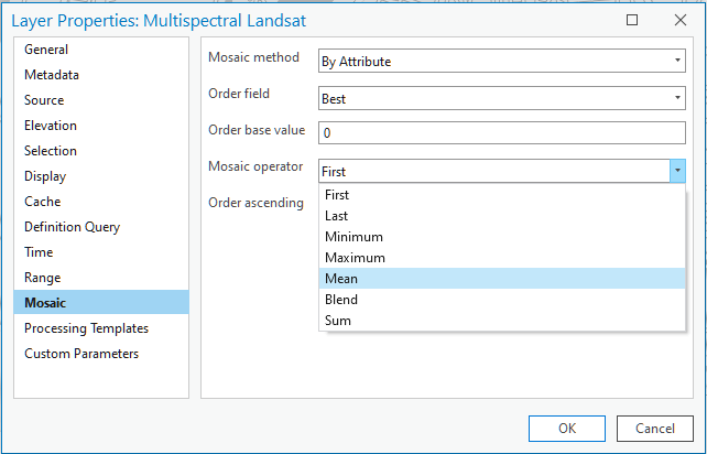
Next, select Mosaic in the Properties pane and choose “Mean” for the Mosaic operator field. You are selecting the mean value because the service contains scenes across decades and for this project you are interested in the long-term average temperature for you study area.
Finally, select Definition Query. Delete any existing query and add a new one where “CloudCover < 0.05.” Apply the query and close the Properties pane. This query will filter out all scenes with more than 5% cloud cover. Clouds and cloud shadows in Landsat scenes adversely impact the results of any analysis. Filtering out cloudy scenes will improve the overall quality of your analysis. Click ‘OK’ to apply the new properties. The online service may take a few minutes to update so be patient.

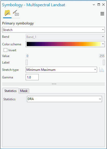
While not necessary, if you wish to visualize the temperature data at this point, you can apply the following symbology settings.
Filter the Service by Location
The last filter step for this input is to filter by location. This step allows you to focus on a smaller area of interest, so Copy Raster executes quickly in the next step. For this example, census polygons from a small area in Seville, Spain, are used to define an area of interest. These Census Section level boundaries are available in Living Atlas.
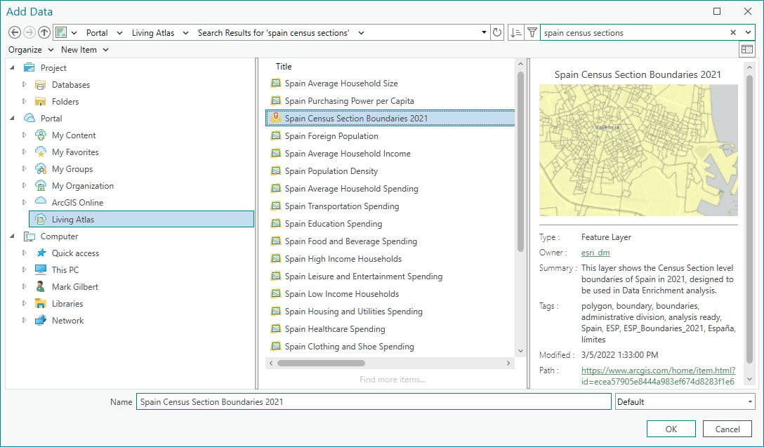
Using the Add Data button, search the Living Atlas for ‘spain census sections’ and add it to the project. Be sure Living Atlas is selected under Portal on the left before typing your search text.
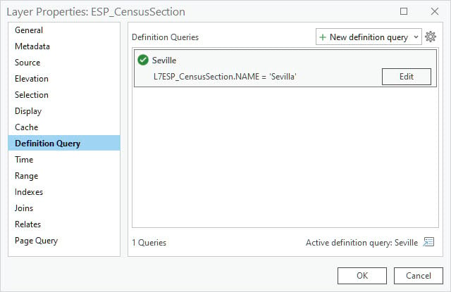
Add a Definition Query to the hosted feature layer you just added to the project. Set the “Name” attribute equal to “Seville” and apply it to limit your area of interest to Seville census polygons. Rename the layer in Contents to something meaningful like “Seville Census Sections”.
Copy Features
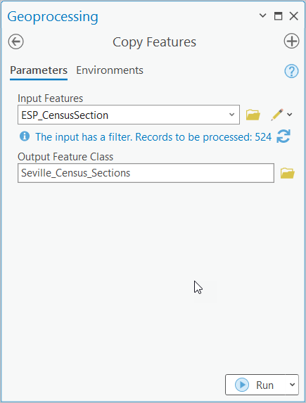
Now that the census sections have been filtered to the area of interest, you will copy the features to a new local feature class for further processing.
Use the Copy Features geoprocessing tool to copy the census sections. Select the filtered hosted feature layer in the Input Features field and give the output feature class a name like “Seville_Census_Sections”.
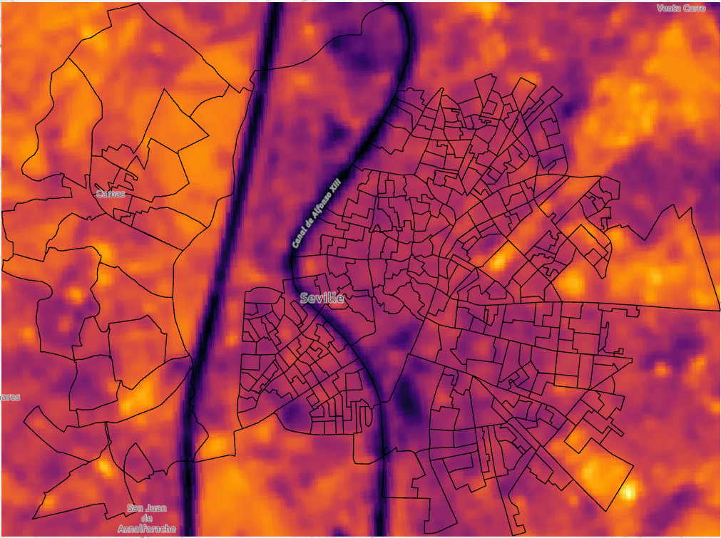
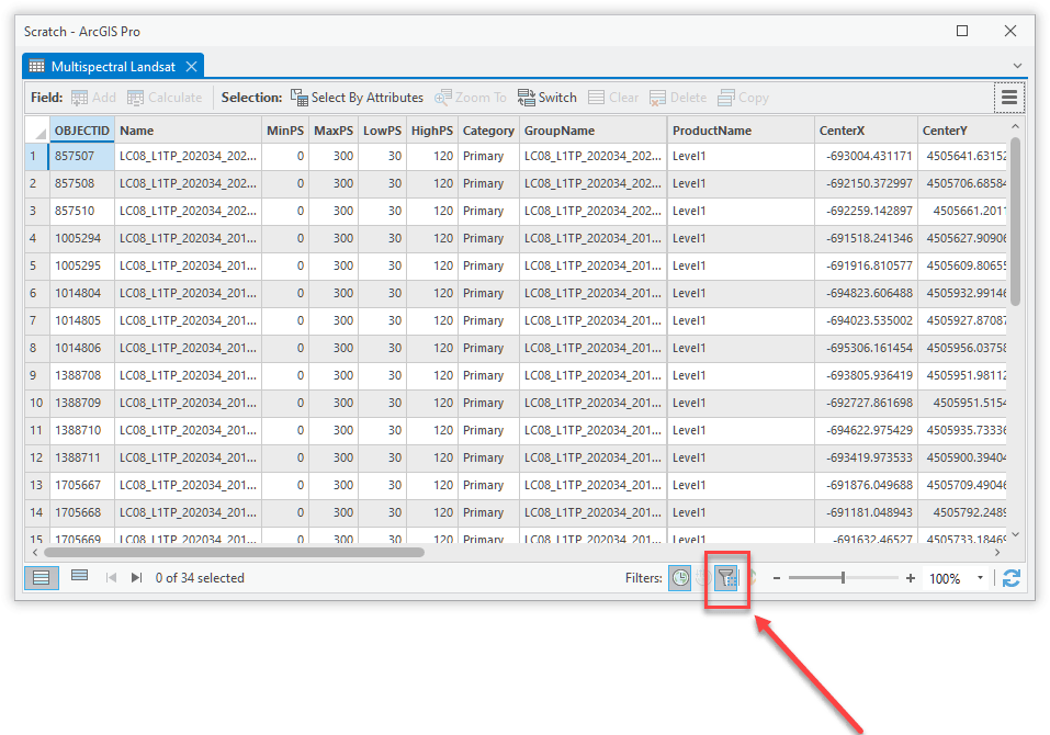
Once the features are copied and added to Contents, zoom the map to the area by right-clicking the features and selecting Zoom to Layer. Next, right-click the Landsat service again and choose Attribute Table. Be sure you have framed your area of interest in the map extent before completing the next step.
The Filter by Extent button is located in the lower-right corner of the Attribute Table.
Click this button to enable the filter based on the current extent of your map.
By changing these properties of the image service, you have configured it to present the average temperature in degrees Celsius across all the scenes in the service. Additionally, you used filtering to limit the scenes to only those with less than 5% cloud cover and spatially limited them to your area of interest.
Copy the Result
Copying this result allows you to focus on your area of interest instead of working with the entire global data set.
Use the Copy Raster geoprocessing tool and copy to TIF format. You will need to enter an output file location that is a folder and give it a name ending in .tif. TIF files may not be output to file geodatabases.
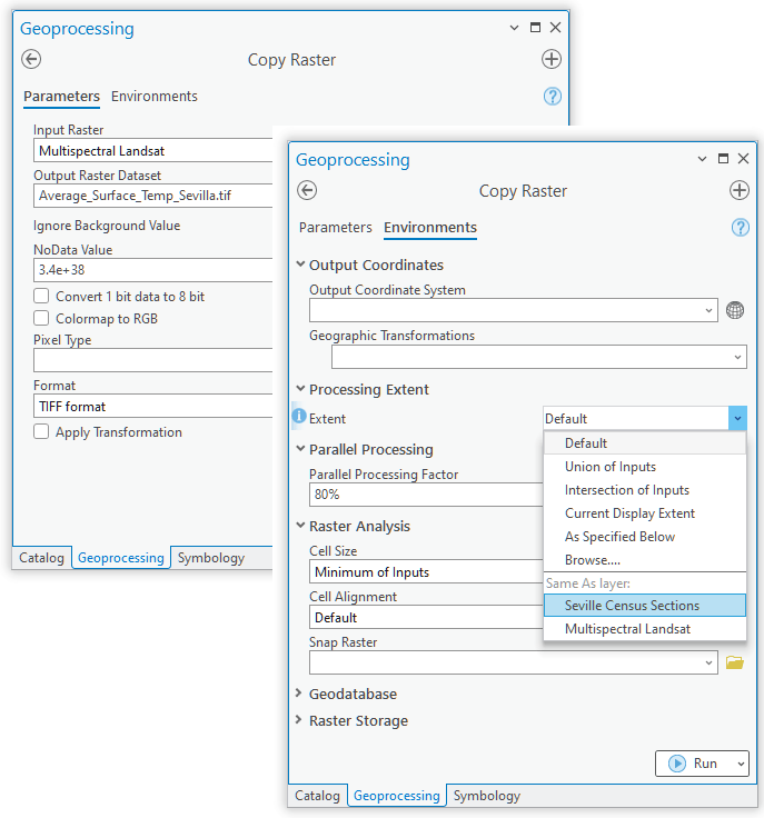
Set the Processing Extent on the tool’s Environment tab by selecting the Seville Census Sections layer. This will clip the raster output to the boundary of the polygons.
Run Zonal Statistics as Table
Now that your area of interest’s surface temperate raster is copied to a local file, you will need to find census polygons for the same location. The example here, uses polygon features from Living Atlas for the area around the Guadalquivir River in Seville, Span. You can use the Zonal Statistics as Table tool to summarize all the temperature values within each census polygon to determine the maximum value. Open the Zonal Statistics as Table Geoprocessing tool. Select the Seville census sections polygon layer for Input Raster or Feature Zone Data, ID for Zone Field, the previous output you just copied as the Input Value Raster and select Maximum as Statistics Type.
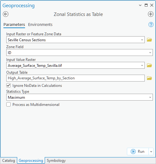
Leave these results in the table for now. In the final blog you will combine the three inputs into a single table for additional processing.
Conclusion
You have now completed the workflow for preparing the first input in the heat resilience index. First, using Living Atlas data, you derived land surface temperature for an area of interest using processing templates on the Multispectral Landsat image service. Then you adjusted properties on the service to filter the scenes by attribute and calculate average values across the filtered scenes. You also applied a spatial filter to limit the scenes to an area around the census boundaries.
Part 2 of this series demonstrates how to prepare the tree canopy input from land cover type. Part 3 explains how to calculate population density from census polygons as well as combining all three inputs into the HRI. Don’t miss them!

Article Discussion: