Various forms of remote sensing data are collected to help understand our planet. Satellite imagery, which captures the reflectance of the Earth’s surface, is a familiar asset within the GIS community and serves as a vital data source for GIS analysis and visualization. Altimetry data is a relatively new addition to the world of GIS and ArcGIS Pro. Altimetry data is collected via satellite sensors that record the elevation of surface features such as canopy height, sea surface height, and ice thickness. This new data and capability present an opportunity for enhanced analysis and understanding. Thanks to NASA’s commitment to open science initiatives—characterized by transparency, accessibility, inclusivity, and reproducibility—these altimetry data are freely and readily accessible to all researchers.
ArcGIS aims to be a comprehensive system capable of handling various forms of remote sensing data, including the processing and analysis of data from altimetry sensors. In this example, CryoSat-2 altimetry data is used for analysis in ArcGIS Pro to quantify the amount of change/loss in the Greenland ice sheet over time. This is a great example of how altimetry data can help support analysis on land. Altimetry data also has effective applications in the ocean environment. The following examples demonstrate how this can be achieved.
The ocean is vast and dynamic. Currently, the number of instruments collecting near-real time in-situ physical oceanographic observations makes it difficult to measure change in the open-ocean with high-accuracy. Satellite altimeters provide a global and precise measurement of ocean surface topography. These instruments operate by transmitting radar pulses to the ocean surface, determining the sensor’s height above the surface by measuring the time taken for the radar pulse to return. The sea surface height is then calculated as the difference between the sensor’s height and the sensor’s height above the surface. These valuable insights allow for monitoring changes in sea surface height, ocean circulation, and weather prediction for tropical cyclones, among other uses.
ArcGIS Pro offers support for various altimetry sensors, including Sentinel 3 SRAL, Sentinel 6, Jason 2 and Jason 3, with the latter two being added recently in the ArcGIS Pro 3.2 Release.
The trajectory dataset
Altimetry sensors gather point data along flight paths, which we refer to as trajectory data. ArcGIS uses a trajectory dataset to effectively manage this type of data. This is like the mosaic dataset model, which organizes a collection of images, the trajectory dataset serves a similar purpose, but managing a compilation of trajectory files containing point measurements. The point sublayer of the trajectory dataset can be utilized as a feature class layer during processing and analysis. You can generate a trajectory dataset from a folder of trajectory files using two geoprocessing tools:
- The Create Trajectory Dataset tool creates a trajectory dataset in a File geodatabase
- The Add Data to Trajectory Dataset tool to is used to load the trajectory files/data into the trajectory dataset. There are different options when importing the trajectory data that allow users to specify the sensor types and the associated variables to be loaded.
Model Sea surface topography using SSH variable
In this example altimetry data from Sentinel-3 is used to map Sea Surface Height (SSH). Sentinel 3 has a two-satellite configuration that offers coverage with a rapid revisit period compared to other altimetry sensors. Sentinel 3 altimetry data can be accessed from EUMETSAT Data Service.
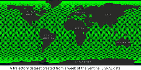
Using a week of level-2 altimetry data a trajectory dataset was created. The trajectory dataset contains an SSH variable that is calculated on-the-fly from the data variables “mean sea surface level” and “sea surface height anomaly”. The SSH variable is computed when “Add Data to Trajectory Dataset” is used to load the altimetry data into the trajectory dataset and the data type “Sentinel 3 SRAL” is selected. Below is the trajectory dataset created from Sentinel 3 SRAL data between 1/2/2022 and 1/8/2022. It contains 394 tracks (green lines) which reference 817,204 observation points.
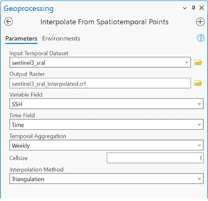
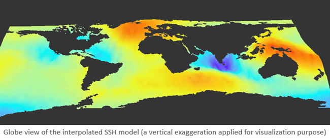
Next, using the “Interpolate From Spatiotemporal Points” tool a SSH raster was produced. To enhance the visualization, the triangulation option for interpolating data was used.
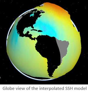
A land mask is also used to clean the pixels on land. The resulting SSH raster dataset was then utilized as an elevation source in 3D, while also functioning as a raster layer draped over the elevation surface. This provides a clear depiction of the peaks and valleys present during this period in the ocean topography.
Analyzing the sea surface height change
In this example data from the Jason 2 and Jason 3 sensors is used to show changes in SSH. The Jason 2 and 3 sensor combination offers continuous temporal coverage from 2008 to the present (Jason 2 – 2008 to 2016 and Jason 3 2016 to present). Access to data from Jason 3 and Jason 2 is available from several sources; in this case, the NOAA NCEI ftp site was accessed due to ease of batch downloading.
To conduct an analysis of sea surface height over an extended period, we utilized two variables: SSH (Sea Surface Height) and SSHA (Sea Surface Height Anomaly). Two independent trajectory datasets for Jason 2 and Jason 3 data respectively were created, each containing the SSH and SSHA variables. Features were then exported to individual feature classes using the “Copy Feature” tool, maintaining them as two separate feature classes for subsequent analysis.
Calculate the average monthly SSHA
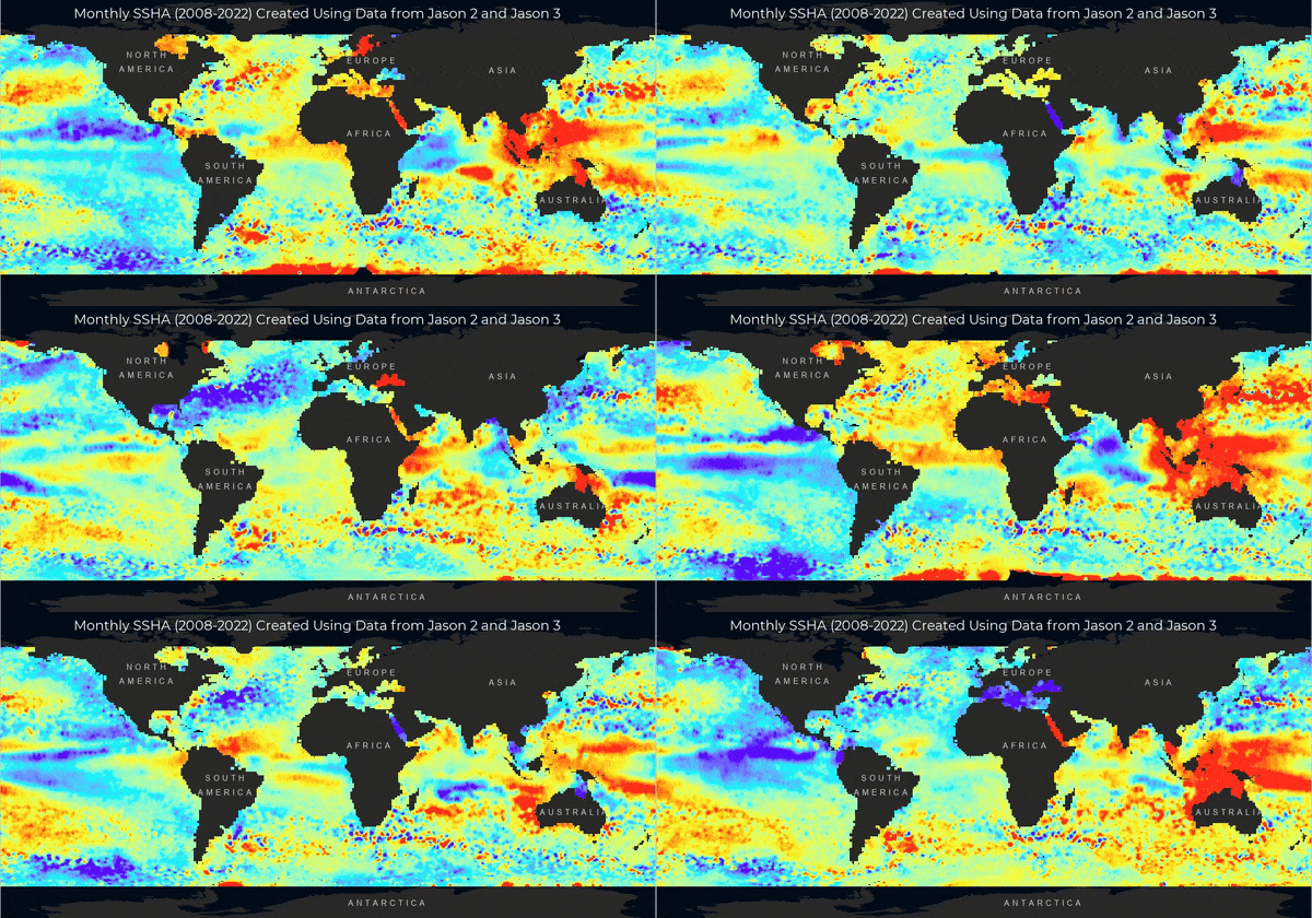
In these steps we use the SSHA data from the Jason 2 and Jason 3 feature classes to create independent multidimensional (time-series) rasters. To do this, we will again use the “Interpolate From Spatiotemporal Points” tool – this time using the IDW option and calculate a monthly SSHA variable for each dataset independently. Next, we merge the outputs from Jason 2 and Jason 3 using the “Merge Multidimensional Raster” tool. The result, animated below, is a monthly time series compilation of both Jason 2 and 3 ranging from 2008 to 2022.
Global average sea surface height change
In this example, the goal is to compute the global average sea surface height utilizing the altimetry data points using both the Jason 2 and Jason 3 feature classes created in the previous step. Once again, the “Interpolate from Spatiotemporal Points” tool is used, this time selecting the “Mean” interpolation method to calculate the monthly averages for each feature class independently. The Mean option computes the average using the observation points within the designated pixel size and time interval, avoiding pixel extrapolation in no data areas and removes the introduction of errors. Below is Jason monthly interpolated mean example created. The valid data area is between -180 and 180 and -60 and 60 (skewed in the polar regions).
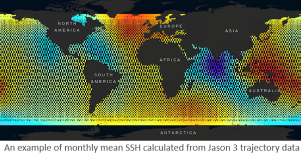
In analyzing the 2016 raster data from Jason 2 and Jason 3 (the one-year overlap maintained for data calibration purposes), we observed a discrepancy of 0.7 meters. Consequently, we applied a correction factor of 0.7 meters to the Jason 2 data prior to merging it with the Jason 3 dataset.
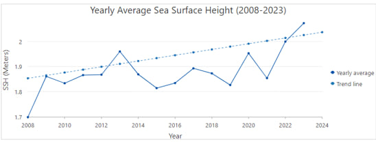
Next, global averages for both monthly and yearly SSH were computed using the “Zonal Statistics as Table” tool; the results are represented as graphs below. This provides the capability to examine seasonal and annual variations, change, and trends in global SSH.

Monitoring significant wave height
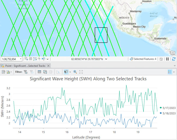
Several of these altimetry sensors offer near real-time measurements of sea surface height, significant wave height, and wind speed, facilitating operational oceanography and climate monitoring. The new Trajectory profile chart capability provides a valuable tool for quickly visualizing near real-time data. The following depicts a comparison of significant wave height from Sentinel 6 over two consecutive days along two distinct tracks.
These examples are intended to help provide insight on how these trajectory tools in ArcGIS Pro can be used for oceanographic analysis. Please feel free to reach out to the blog authors if you have questions, comments, or feedback.


Article Discussion: