Introduction

Creating data for the voxel layer can be an intimidating process. The process of creating source data (NetCDF) from a table is laid out in this blog. In collaboration of the Technical University of Darmstadt, soil permeability data was collected, processed and visualized as a voxel layer.

Data Collection

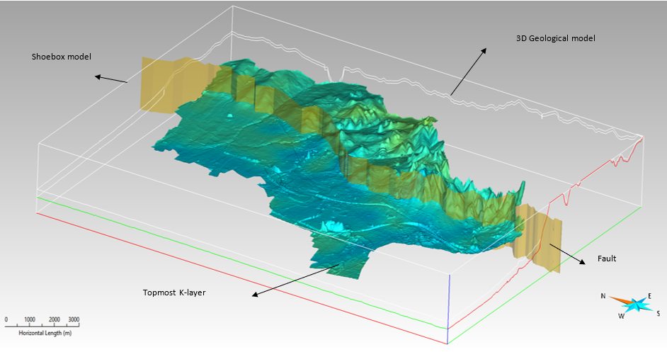
The 3D geological model (SGrid) for the study area is generated using the software SKUA-GOCAD (Emerson Paradigm Holding LLC). The model describes the aquifer distribution of the study area. The delineation of the aquifers is based on a voxel model parameterized with petrographical descriptions and kf-classes. In addition, measurements describing the groundwater level are utilized. A north-south trending sub-vertical fault is also included in the model. In the eastern fault block the model covers the upper 10 meters, in the western fault block the upper 30 meters. In order to provide content in the NetCDF format, which is needed for a visualization in ArcGIS Pro, the overall framework of the model requires some adjustment before the data can be exported to ASCII format. A shoebox model must be generated in SKUA-GOCAD; it contains the original geological model.  The image below illustrates the cage geometry of the original model included within the extent of the shoebox model, with the topmost K-layer of the geological model being displayed along with the major fault in the study area.

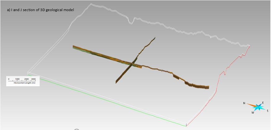
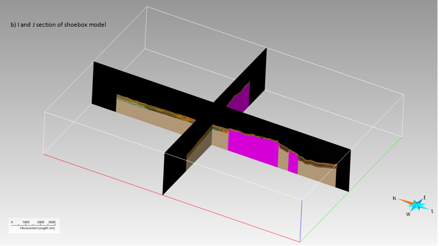
The main difference between the two models (shoebox and geological) is the geometry of the K-layers. The K-layers in the original 3D geological model follow the morphology of the topographic surface. In contrast, the K-layers in the shoebox model are horizontal.  The cell resolution of the horizontal K-layers is 25m x 25m x 2m along each (X, Y, Z) direction respectively. Each horizontal K-layer now receives properties from the original model by a transfer. Above the topographic surface, No data value (-99999 or -9999) is assigned to the cells since every single cell needs a value. In addition, in the eastern fault block the lithology and permeability are extended to 30 meters to match the total depth of the western block, leading to an overall regular gridded volume.

In this example, the properties were transferred using the command “Transfer Property > From Nearby Grid Node or Cell” in SKUA-GOCAD. The command transfers property from an object to another. The object can be an SGrid, a Voxel or a Solid. The transferred values are snapped from the server cell to client node which it resides in. If the server is a cell-centered SGrid or a Voxel with a block-interpolated property; the transferred value is interpolated from nearby server nodes in all other cases. After this step, the K-layers are converted to triangulated surfaces. The triangulated surfaces contain coordinates, depth, K-layer identifier, permeability, lithology and fault identifier as properties. These triangulated surfaces are exported separately as ASCII files for the processing stage using a Python script and later for visualization in ArcGIS Pro as a voxel layer.

Processing ASCII to NetCDF with Python

The modules needed to process the data are numpy, netCDF4, and pandas. The aforementioned K-layers exported from SKUA-GOCAD in this example are written out as one layer per ASCII text file. Therefore, all text files must first be collected which includes the need for the standard module os as well.

folder is a variable which indicates the folder directory where the ASCII files are located. files holds a list of all files in the directory with their full path appended before the file name.

import netCDF4
import os
import numpy as np
from netCDF4 import  Dataset
import pandas as pd
 
# Folder path
folder = r'C:\temp\myData'

# Collect all text file paths
files = [os.path.join(folder,f) for f in os.listdir(folder) if os.path.isfile(os.path.join(folder, f))]

The ASCII file is delimited by a single space, and a newline separates entries. Using the read_table function from the pandas module, a dataframe is created to hold the first K-layer entry. The size variable is used to verify that each K-layer have an equal number of entries, due to the requirement of having equally spaced gridded data.

# Create initial dataframe
dfPoints = pd.read_table(files[0], delimiter = ' ') 

# All files need consistent size
size = dfPoints.size

Now that all files are collected into a list, they must be processed using a for loop starting at the first index (second element) of the list, since the zeroth index (first element) was already added to the dataframe. A dataframe buffer is created each iteration of the loop. If the size of the buffer is not equal to the size variable, we continue to the next file in the list. If it is equal, then it is appended to the original dataframe, dfPoints. The number of entries in this dataframe will be equal to the total number of entries across all valid files.

# Put all data into dataframe
for i in range(1, len(files)):
  dfBuffer = pd.read_csv(files[i], delimiter = ' ')
  if(dfBuffer.size != size):
    continue
dfPoints = dfPoints.append(dfBuffer, ignore_index = True)

Since the data is not guaranteed to be in any kind of order, the dataframe is sorted using the sort_values function. This data is sorted first by the Z coordinate, then Y, and finally X. Voxel layers have requirements for dimension order, (X,Y,Z,T) or (T,Z,Y,X) with the T and Z dimension being removeable, but at least 1 of them is required to be present in the data.

The domains of each dimension must also be extracted from the dataframe. Using the index location, or iloc operator, the raw values are accessed. Using the numpy function unique a list of unique values for each dimension is created and then sorted.

# Sort the values by Z, then Y, then X
dfPoints = dfPoints.sort_values(by=['Z','Y','X'])

# Create domain for longitude, latitude, and Z
xDomain = np.sort(np.unique(dfPoints.iloc[:,0].values))
yDomain = np.sort(np.unique(dfPoints.iloc[:,1].values))
zDomain = np.sort(np.unique(dfPoints.iloc[:,2].values))

Now the data is processed and mostly ready to be added to a NetCDF file. A output file must first be created using the Dataset constructor. Dimensions of the NetCDF file are set using the createDimension function for X, Y, and Z. The length of each domain must also be specified.

# Create NetCDF
outDataSet = Dataset('myOutput.nc', 'w', format = 'NETCDF4')

# Create dimensions
outDataset.createDimension('z',len(zDomain))
outDataset.createDimension('y',len(zDomain))
outDataset.createDimension('x',len(zDomain))

The createVariable function is used to create a variables in a NetCDF file. Each dimension must have a variable associated with it, which contains the values in their respective domains. Other variables, such as Lithology and Predicted KF in this case, have multiple dimensions associated with it. For example, ncLithology has the Z,Y,X dimensions, therefore the number of entries for ncLithology will be the length of each dimension multiplied together. fill_value is a property of the variable which indicates what value was used to fill missing data.

# Create variables
ncZ = outDataset.createVariable('z', np.float32, 'z')
ncY = outDataset.createVariable('y', np.float32, 'y')
ncX = outDataset.createVariable('x', np.float32, 'x')
ncPredictedKF = outDataset.createVariable('Predicted_kf', np.float32, ('z', 'y', 'x'), fill_value = -99999)
ncLithology = outDataset.createVariable('Lithology', int, ('z', 'y', 'x'), fill_value = -9999)

Now that the variables for the NetCDF file are created, the values in the dataframe that were processed earlier must be assigned to the variables. Using the [:] operator, the values processed are assigned to the NetCDF variable values. For the variables which have three dimensions, the [:,:,:] is the same operator, but implies that there are three dimensions to the array. Variables more than one dimension must have their dataframe values be reshaped to match the size of the multidimensional array which was allocated for the output. Numpy has a reshape function which allows this to be accomplished. The second argument of reshape is a tuple of values, and in this example the tuple consists of the length of each dimension, Z,Y,X.

# Assign values
ncX[:] = xDomain[:]
ncY[:] = yDomain[:]
ncZ[:] = zDomain[:]
ncPredictedKF[:,:,:] = np.reshape(
  dfPoints['Predicted_kf'].values,
  zDomain.shape[0], yDomain.shape[0], xDomain.shape[0]
)
ncLithology[:,:,:] = np.reshape(
  dfPoints['Lithology'].values,
  zDomain.shape[0], yDomain.shape[0], xDomain.shape[0]
)

With the values added, some attribute information can be added to each variable. Attributes such as long_name and units give information but do not change the way the layer draws. Other attributes, such as positive, will change the way the layer draws. positive gives the direction of the data, and in a voxel layer this attribute determines the vertical exaggeration direction. Global attributes can also be assigned, which apply to the entire dataset. In this case, esri_pe_string is used to the coordinate system. After adding attributes, the output NetCDF is closed.

# Assign attributes
ncPredictedKF.long_name = 'Predicted_kf'

ncLithology.long_name = 'Lithology'

ncZ.positive = 'up'

ncY.standard_name = 'projection_y_coordinate' 
ncY.units = 'm' 

ncX.standard_name = 'projection_x_coordinate' 
ncX.units = 'm' 

outDataSet.esri_pe_string = 'PROJCS["ETRS_1989_UTM_Zone_32N_7stellen",GEOGCS["GCS_ETRS_1989",DATUM["D_ETRS_1989",SPHEROID["GRS_1980",6378137.0,298.257222101]],PRIMEM["Greenwich",0.0],UNIT["Degree",0.0174532925199433]],PROJECTION["Transverse_Mercator"],PARAMETER["False_Easting",2500000.0],PARAMETER["False_Northing",0.0],PARAMETER["Central_Meridian",9.0],PARAMETER["Scale_Factor",0.9996],PARAMETER["Latitude_Of_Origin",0.0],UNIT["Meter",1.0],AUTHORITY["Esri",102328]]' 
outDataSet.close()

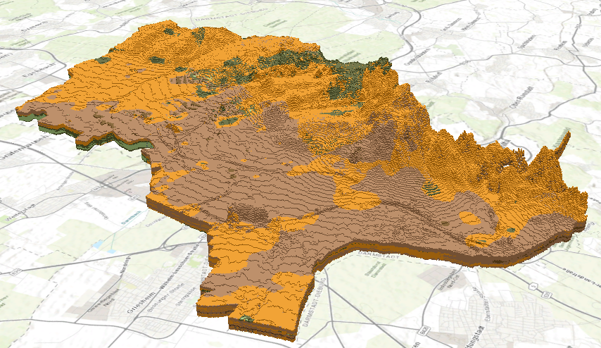
The resulting NetCDF can be added to a voxel layer for analysis and exploration, as seen below. For more information on adding a NetCDF to a voxel layer, please see add a voxel layer to a local scene.

About the Authors:

Rouwen Lehne

Hessian Agency for Nature Conservation, Environment and Geology (HLNUG), TU Darmstadt

Rouwen is a geologist working for the Geological Survey of Hesse (Germany). He is very interested in geodynamic processes and how information about geology can contribute to sustainable action. Of particular interest is the urban space and thus the synopsis of various specialized information in 3D space. To work on such questions he uses geoinformation systems and tools for 3D modeling as well as for 3D visualization.

Sonu Roy

Sonu is pursuing her second Master’s degree in Tropical Hydrogeology and Environmental Engineering at TU Darmstadt, Germany. She started her career as a Geomodeler in Oil and Gas Industry. She is doing her Master’s thesis in the field of Geomechanics. She believes that the future lies in renewable energies and wants to contribute in the research sector.

About the author

Richard Vargas

Richard is a Product Engineer (SDET) on the 3D Scene Layers Team at ESRI. In this role he works on multidimensional voxel and 3D object layers, as well as a maintainer for the ESRI I3S specification. Richard has a Bachelor of Science in Computer Science from California State University San Bernardino. Outside of work, Richard likes to indulge in video games, fiddle with the guitar, and go on hikes.

Connect: