A Workflow for Creating Discrete Voxels

Note: In ArcGIS Pro 3.1 and later, it is recommended to use the Nearest Neighbor 3D tool to accomplish the workflow described in this blog.

First available in ArcGIS Pro 2.6, a voxel layer represents multidimensional spatial and temporal information in a 3D volumetric visualization. Voxel layers are based on data stored in a netCDF file.  In ArcGIS Pro, the netCDF file can be created from a geostatistical layer or a space-time cube. A typical workflow is to take points with attributes representing a continuous variable (for example, temperature), perform 3D kriging using the Empirical Bayesian Kriging tool, and convert the output geostatistical layer to a netCDF file using the GA Layer 3D To NetCDF tool. This netCDF file can be added to a scene in ArcGIS Pro as a multidimensional voxel layer.

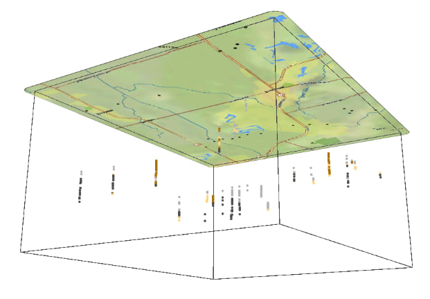
But what if the attribute of your points represents discrete categories (for example, soil type) rather than a continuous variable like temperature? 3D kriging expects the input data to have a continuous attribute for interpolation, but it can be configured to perform nearest-neighbor interpolation. In nearest-neighbor interpolation, the value at a new location (a location where you don’t have a sample point) is assigned the value of the nearest input point in 3D space. This allows you to visualize and explore the categories of the points as a full voxel cube in 3D.

Perform Nearest-Neighbor Interpolation

This blog will provide the configurations to perform nearest-neighbor interpolation, but it will not explain the parameters or what they mean. To learn about 3D interpolation and all parameters of Empirical Bayesian Kriging 3D, consider completing this lesson: Interpolate 3D oxygen measurements in Monterey Bay.

In the example below, we’ll use soil type recorded at various depths in boreholes located just west of St. Louis, Missouri. The data were downloaded and processed from the ArcGIS Code Sharing site and contributed by Jennifer E. Carrell, Illinois State Geological Survey, University of Illinois at Urbana-Champaign. The 3D points contain a subset of the soil types (formations) in this region: clay, loam, sand, and shale.

1. Convert soil type categories to a number (integer) field.

• The Empirical Bayesian Kriging 3D tool only accepts a numeric value to interpolate. Each unique soil type must be converted to a unique integer (for example, clay to 0, loam to 1, etc.). Hint: Use the reclassify helper function in the Calculate Field tool if you have many categories to convert.

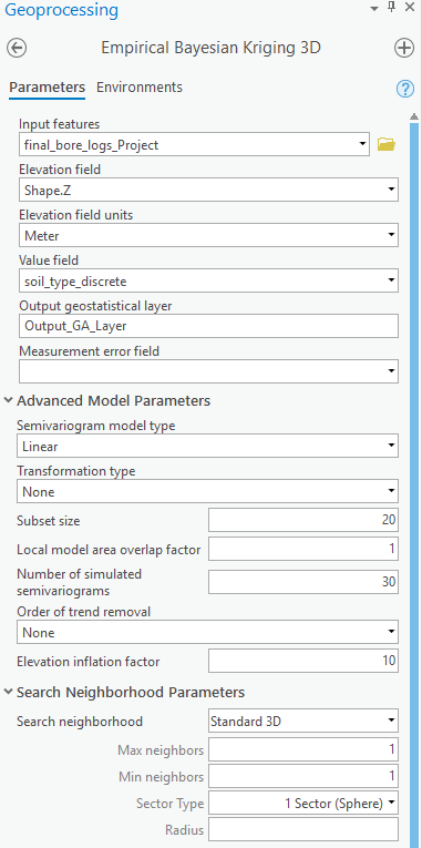
2. Configure settings to perform nearest-neighbor interpolation. Some parameters are required, but most are to avoid as many unnecessary kriging calculations as possible.

• Using the integer field created in the previous step, run the Empirical Bayesian Kriging 3D tool with the following parameters, leaving all other optional parameters at their default values:
  • Semivariogram model type: Linear
  • Subset size: 20
  • Number of simulated semivariograms: 30
  • Elevation inflation factor: 1 (or the same value as the vertical exaggeration on the input layer)
  • Max neighbors: 1
  • Min neighbors: 1
  • Sector type: 1 Sector (Sphere)

3. Add the output netCDF file from the previous step to a local scene as a voxel layer.

• Make sure the coordinate system of the local scene is the same as the input points.
• From the Add Data drop-down, choose Add Multidimensional Voxel Layer.
• Browse to the location of the netCDF file created in the previous step.
• Change the Data Type to discrete.
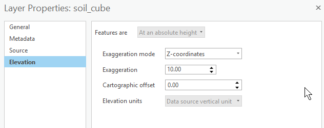
• Once the voxel layer is created, you will need to change its exaggeration mode and value for the voxel layer to align with the points in 3D. The exaggeration mode should be Z-coordinates and the value should match that of the input points.

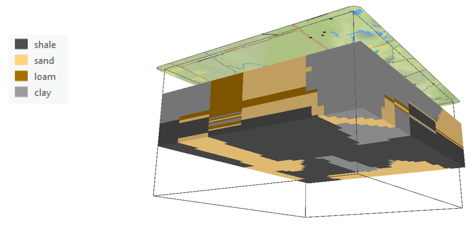
Discrete Voxel Layer in a Scene

The voxel layer now displays in the local scene and aligns with the input points. Each individual voxel within the voxel layer contains the value of the soil type of its closest neighbor in 3D. You can explore voxel layers in many ways, including advanced transparency, sectioning, isovolumes, and animations. Learn more about the capabilities and options of voxel layers.

Considerations and Limitations

1. Nearest-neighbor (NN) interpolation should be considered a display option rather than an interpolation method. Unlike other interpolation methods that mathematically estimate continuous values at new locations, NN interpolation is a simple assignment algorithm.
2. The quality of the visualization heavily depends on your sampling plan. It is best to have samples evenly distributed throughout your study area in 3D.
3. This technique is most appropriate as an initial visualization and may not work well in poorly stratified or highly interfingered formations.

Acknowledgements
Thank to Eric Krause (Spatial Statistics Team) for configuring the parameters for nearest-neighbor interpolation.