Wishing out loud:
“Wouldn’t it be great to define a series of processes you want to apply to an image – or suite of images – and see the results immediately?”
“Then analyze those results and make some informed judgement calls on adjusting parameters to interactively optimize outcomes?”
“And not have to store and manage all the intermediate datasets that contribute to your final products?”
News Flash – You can achieve all these needs by using raster function templates in ArcGIS Pro! This tutorial introduces the concepts of building a raster function template to support a processing workflow for assessing vegetation coverage and relative health.
Assess vegetation for wildlife habitat
The Sacramento National Wildlife Refuge was established in 1937, and provides critical refuge and breeding habitat for migratory birds and other wildlife as well as management for endangered, threatened, and sensitive species. The refuge supports over 300 species of birds, and the huge wintering concentrations of over a million waterfowl is truly awe inspiring!
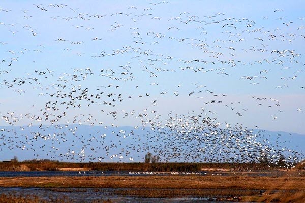
The refuge also serves to alleviate crop damage from wildlife along the Sacramento River valley, which is an important portion of the Pacific Flyway between North America and South America. Evaluating the coverage and relative health of both natural vegetation and crops in the surrounding area helps to balance the requirements and management of natural wildlife and agriculture landuse.
Use interactive on-the-fly image processing to achieve quality results
One of the coolest and most useful image processing capabilities in ArcGIS Pro is on-the-fly dynamic processing. Create and modify raster function processing chains using the intuitive raster function editor, and examine image processing results in near real time as you roam and zoom layers in the map viewer. Another advantage is there is no need to store and manage intermediate processing results to disk.
What you see is what you get as the result of your processing chain. See an issue or the results are not exactly what you were expecting? No problem, just go into the Raster Function Editor, modify any number of parameter for any of the functions and see the updated results in real time. When optimal results are achieved, save the processing chain as a raster function template, and save the results to disk or cloud storage.
This tutorial will get you started with on-the-fly processing using raster functions to evaluate vegetation coverage and relative health in the Sacramento River valley. You will generate a vegetation index and assign a color map to visualize the results. The workflow has the following five steps:
- Download the sample data.
- View the image layer.
- Compute the vegetation index.
- Classify the vegetation results.
- Assign a color scheme for visualization.
Add the tutorial data to your project
The data packaged for this tutorial includes a subsection from a Landsat8 scene collected on June 8, 2018, along with the refuge boundary data.
1. Download the tutorial data and save it to your machine. Unzip the files.
2. In ArcGIS Pro, create a new project using the Map template and sign in to your ArcGIS Online account if necessary.
3. Set up your project:
a. On the Map tab on the main Pro ribbon, Layer group, click the Basemap drop-down arrow and select Imagery. This will replace the default basemap with world imagery.
b. On the Insert tab, click Add Folder which opens a dialog for you to navigate to the folder where you copied the tutorial data. Click OK.
c. On the View tab, click Catalog pane. Pin the pane.
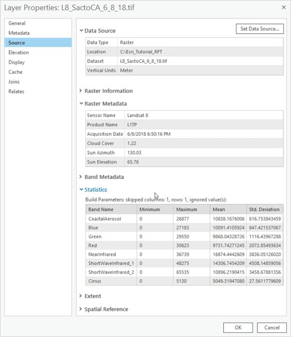
4. In the Catalog pane, click the Folders expander arrow to display the directory where you copied the tutorial data. Right-click the L8_SactoCA_6_8_18.tif layer and select Properties, which opens the Properties dialog. Select Source in the panel to display detailed Raster Information, Raster Metadata, Band Metadata, image Statistics, Extent and Spatial Reference information. All these image file properties are derived from the source Landsat 8 metadata. Explore the different types of metadata associated with the image data.
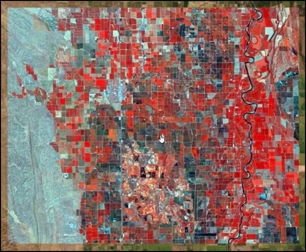
5. The image is displayed as a natural color image, using the red, green and blue channels. To change the band combination to color infrared, click on the Appearance tab on the main Pro ribbon. In the Rendering group, click the Band Combination drop-down arrow and select Infrared. Notice that the label for the red display channel of the image in the Contents pane changed from Red to Infrared.
NOTE: Optionally, you can change the band combination by right-clicking the red color chip for the L8_SactoCA_6_8_18.tif layer in the Contents pane, and select NearInfrared.
The image is displayed as color infrared, where bright red indicates vigorous vegetation. Notice that, with the color infrared display, you can more easily identify areas of healthy or dense vegetation compared to other features. For example, you can quickly pick out the river from the surrounding vegetation. This is because water strongly absorbs energy in the near infrared (NIR) portion of the electromagnetic spectrum, so it appears very dark next to the healthy vegetation which strongly reflects NIR light and appears bright red.
Compute the vegetation index
Next you will use a vegetation index to delineate areas of dense healthy vegetation. In image analysis, an index is a combination of band reflectance values that help you identify specific features in your image based on the reflectance and absorption qualities of that feature. Healthy green vegetation absorbs light in the red band, while it reflects green and NIR light. We will use this information to calculate the Soil Adjusted Vegetation Index, or SAVI, so we can understand more about the vegetation characteristics in the Sacramento River valley.
1. Click the image layer in the Contents pane to activate it. Select Imagery on the Pro main ribbon. In the Analysis group, click Raster Functions. Pin the Raster Functions pane.
2. Type “band” in the search and click on the Band Arithmetic raster function in the Math category. The dialog for the function will be displayed.
Note: Click on the ? in the Band Arithmetic raster function dialog to display the function help. Many types of out-of-the-box vegetation indices are described. Of course you can also create your own custom math function or algorithm using this raster function.
3. Set the parameters for the Band Arithmetic function:
a. Raster – click the drop-down arrow and select L8_SactoCA_6_8_18.tif layer.
b. Method – click the drop-down arrow and select SAVI (Soil Adjusted Vegetation Index)
c. Band Indexes – type 5 4 0.33, which are the band numbers for the Landsat 8 NIR and red bands, and an estimate of green vegetation cover.
d. Click Create new layer
The resulting single band SAVI layer is loaded into the Contents pane and displayed in the map viewer. The name of the applied raster function is a prefix to the source data filename, in this case it is Band Arithmetic_L8_SactoCA_6_8_18.tif.
While the data is 32 bit floating point format, it is scaled to 8 bit in order to display it. Bright areas exhibit full vegetation coverage and high relative vigor. Dull or dark areas exhibit non-vegetated areas such as bare soil or water bodies.
NOTE: If the result is a gray block, select the layer in the Contents pane, open the Appearance tab on the main ribbon and select DRA from the Rendering group.
Categorize the vegetation results
You can visually identify the areas that show up as healthy, dense vegetation. Now, you’ll group your results into four distinct categories for interpretation.
1. In the Raster Function pane, search for “remap” and click to open the Remap raster function in the Reclass category.
2. Set the parameters to remap the values of the layer:
a. Raster – click the drop-down arrow and select the Band Arithmetic_L8_SactoCA_6_8_18.tif layer.
b. Remap Definition Type – choose List since you will be manually listing the different categories.
c. Fill out the list using the values below:

d. Check the box to Change Missing Values to NoData.
e. Click Create New Layer.
The resulting single band image shows categorical data on a scale from 1-4, where 1 represents areas with very low SAVI values, indicating little to no vegetation, and 4 represents high SAVI values or dense, healthy vegetation. The name of the layer is Remap_Band Arithmetic_L8_SactoCA_6_8_18.tif.
3. Click on the name of the layer in the Contents pane to rename it to SAVI_Categorized.
Assign a color scheme to the vegetation Index
You can assign a color scheme to the SAVI_classified layer by following the steps below.
1. Select the layer in the Contents pane. In the Pro main ribbon, click Appearance, then click the Symbology icon in the Rendering group. The Symbology pane will open.
2. Click the drop-down arrow on the Primary symbology to select Classify as the symbology type. Choose Yes to compute the histogram.
3. By default, the four classes you chose when using the Remap function display in the symbology table. Click on each color chip to change the colors to a more appropriate color scheme. You can also change the label to be easier to interpret. Use the following intervals as a guide:
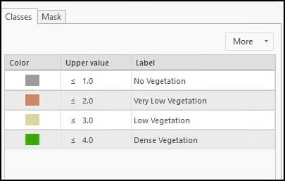
The colors chosen for no vegetation were Grey 30% for no vegetation, Nubuck Tan for very low vegetation, Lime Dust for low vegetation and Leaf Green for dense vegetation.
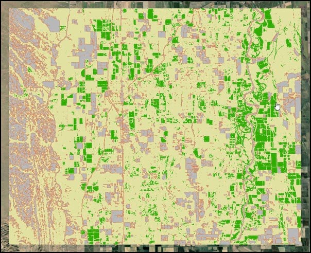
4. To review the chain of functions used to accomplish this result, right-click on the SAVI_Categorized layer in the Contents pane and select Edit Function Chain.
The Raster Function Editor window opens and loads the function chain used to process this layer. You can modify the parameters of the existing processes by double-clicking on the functions, or you can add functions to the chain to extend your process.
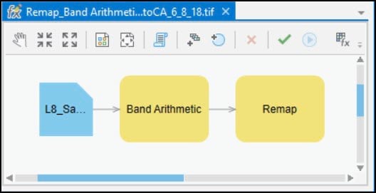
5. Double-click on the Remap function to see the parameters you set earlier. Click Cancel to close.
6. Save the raster function template by selecting the functions you want in your processing chain (Ctrl-click each function, or select by rectangle in rubber band mode) and right-click on one of the active selected functions and choose Export as template. A new raster function editor window will open and load the raster function chain. Click Save As to save the raster function processing chain as a RFT with a name and location.
7. Up to this point in your image processing workflow, all the processing has been done on-the-fly and no new data has been created on your local disk. As an option, you can save the results as a new raster dataset to disk.
Right-click the layer in the Contents pane, select Data, then Export Raster. Specify an Output Raster Dataset, Output Format and click Export.
Summary
Wildlife managers use SAVI and other vegetation index information to assess the amount and vigor of vegetation within the refuge together with the bird population counts to estimate demand for forage. When demand exceeds capacity, the birds seek forage on nearby productive agriculture land, which is also identified by vegetation index information. Cooperative Agriculture – partnering with farmers and ranchers to meet wildlife management objectives – is a long-standing practice on national wildlife refuges. Farmers and wildlife managers work together to improve natural habitat, and farmers are compensated appropriately for their contribution to wildlife resources.
In this tutorial, we examined the SAVI assessment of coverage and relative health of vegetation for the Sacramento River valley and surrounding agricultural land. Raster functions enable dynamic image processing capability and displays results in the map viewer as you pan and zoom the image. Make adjustments to the functions and visualize the results immediately. This helps support wildlife and farm management practices based on analytical information using intuitive image processing techniques.

Commenting is not enabled for this article.