Use a Raster Function to Derive Lack of Tree Canopy

This blog is part 2 of 3 in a series that walks through the steps to use a global collection of ready-to-use geographic information to derive input variables needed to calculate a heat risk index (HRI). Local communities can use the resulting intervention-focused map to prioritize census tracts for tree planting as one mitigation against urban heat islands.

Part 1 of this series explored step #1 of the heat risk index workflow, deriving land surface temperature from multispectral Landsat data. Now we continue with step #2, calculating the lack of tree canopy using a derived tree cover data set.

Refresh your memory of Part 1 and continue the workflow below.

Add Data from the Living Atlas of the World

Similar to the first blog, we need the appropriate source data from ArcGIS Living Atlas of the World. The second input for the HRI is the lack of tree canopy. This is derived from the European Space Agency WorldCover 2020 Land Cover imagery service. Using the Add Data button, search the Living Atlas for “ESA WorldCover” and add it to the project. Be sure Living Atlas is selected under Portal on the left before typing your search text.

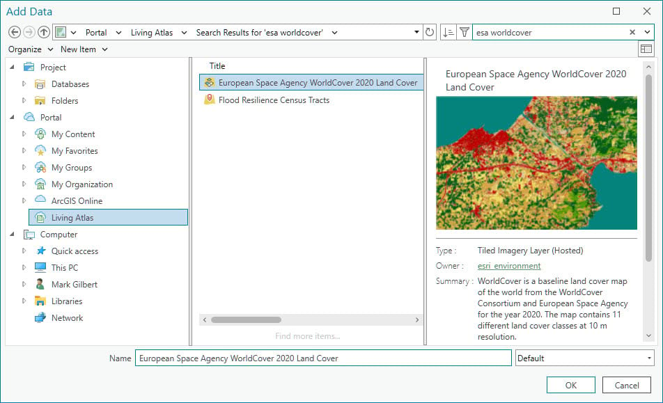
ESA WorldCover is a global landcover data set utilizing 11 different land cover classes. The following steps will describe how to isolate only the tree cover pixels.

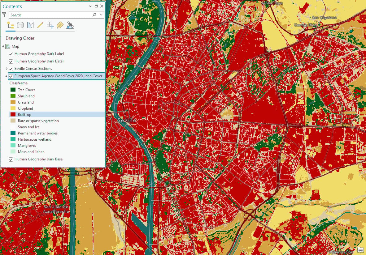
Isolate the Tree Cover Classification

The lack of tree canopy is calculated using the formula ‘100 – Percent Tree Canopy’. This requires you to isolate the WorldCover data to only pixels classified as Tree Cover. The Item Details page for the image service indicates that tree cover pixels have a value of ’10’. The Remap Raster Function allows you to remap all pixels so that only the tree cover remains.

With the ESA WorldCover item selected in Contents, click the Imagery tab on the Ribbon and then click Raster Functions.

Open the Remap Raster Function either by searching for it or expanding the Reclass heading and selecting it. Next, complete the data entry pane displayed below and click the Create new layer button.

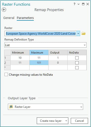
The raster function output will display as a new layer in Contents. This raster function remaps tree cover pixels to a value of 1 and everything else to 0.

Copy the Result

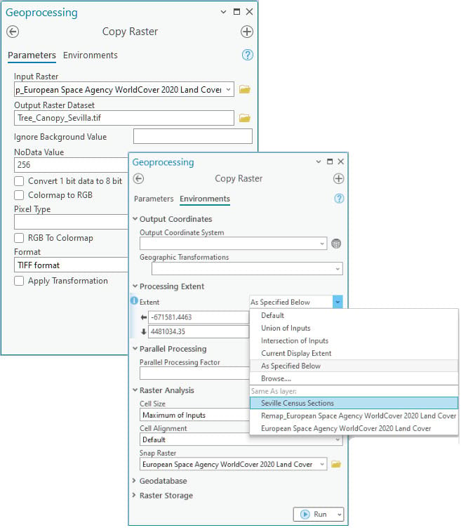
Copying this result allows you to focus on your area of interest instead of working with the entire global data set. If you have been following this blog series, you should already have the Seville Census Sections in your project for the next step. If not, review the section titled “Filter the Service by Location” in blog #1, here, for the steps to add and filter the census polygons.

Use the Copy Raster Geoprocessing tool and copy to TIF format. You will need to enter an output file location that is a folder and give it a name ending in .tif. TIF files may not be output to file geodatabases.

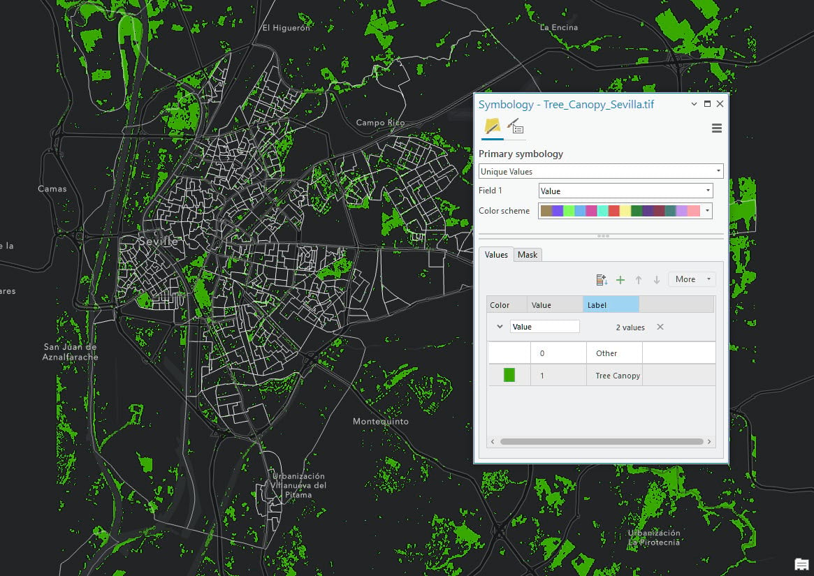
While not necessary, if you wish to visualize the tree canopy data, you can apply the following symbology settings.

Run Zonal Statistics as Table

Now that the tree canopy raster covering your area of interest has been copied to a local file, you are ready for the next step. You will use the same census polygons for Seville, Spain that you used in the previous blog. You can find it here if you need to go back and review it.

You will use the Zonal Statistics as Table tool to count the number of tree cover pixels within each census polygon. The tool also counts the total number of pixels within each zone (polygon), so you can calculate the percentage of the polygon pixels covered with trees.

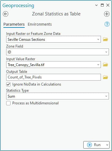
Open the Zonal Statistics as Table Geoprocessing tool. Select the Seville census polygon layer for Input Raster or Feature Zone Data, ID for Zone Field, the previous tree canopy output you just copied as the Input Value Raster and select Sum as Statistics Type.

Calculate Lack of Tree Canopy

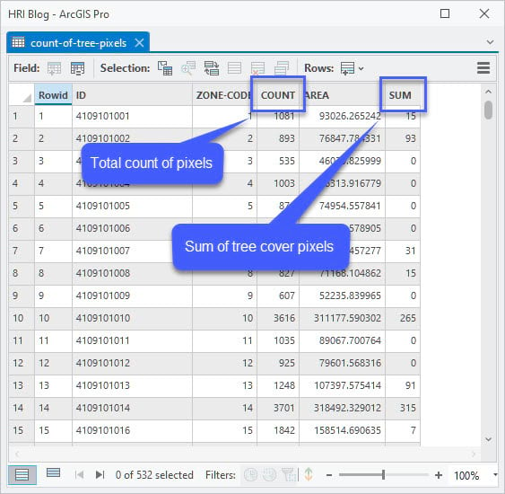
The results of the Zonal Statistics tool look something like the image below. There is a count of total pixels within each polygon zone called ‘COUNT’ and the sum of tree cover pixels called ‘SUM. ‘ By remapping the tree cover pixels’ values to 1’s and everything else to 0’s in the previous step, summing the values will give the count of tree cover pixels. This allows you to divide the ‘SUM’ attribute by the ‘COUNT’ attribute to get a percentage of each polygon that is tree cover.

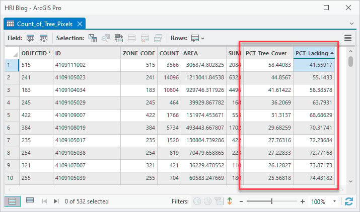
Use the Calculate Field tool and the following formulas to calculate the percent tree cover and percent lacking tree cover for each census polygon.

After you run these calculations, the attribute table should look like this.

Leave these results in the table for now. In the final blog, you will combine the three inputs into a single table for additional processing.

Conclusion

This completes the workflow for preparing the second input to the HRI. First, you isolated tree cover pixels in the ESA WorldCover 2020 Land Cover date set using Living Atlas data and extracted the data for your area of interest. Next, you summarized the count of tree cover pixels falling within each census boundary. Finally, you calculated the percentage of each polygon that contains tree pixels, and that lacks tree pixels.

Part 3, and the final blog of this series, explores how to calculate the population density for each census polygon and how to combine all three inputs into the HRI.