Research has shown that communities of color, Indigenous communities, and low-income communities are disproportionately impacted by the health burdens of air pollution. To look at this issue more closely, we’ve collaborated with researchers from Harvard School of Public Health and Senator Cory Booker’s team to create an ArcGIS StoryMaps story to visualize the results and in turn, promote public awareness and bring a call to action.
Among the findings of this research is a focus on the presence of Particulate Matter (PM) and particularly, PM 2.5. PM 2.5 are tiny particles in the air that can contribute to asthma, heart disease, decreased lung function, and even death. In order to better understand the impact of PM 2.5, we’ll conduct an initial analysis and visualize the results. Let’s take a look.
In the example below (Figure 1), the top map shows PM 2.5 levels across the United States. Areas that are symbolized with the darkest blue represent the highest levels of air pollution. The bottom map shows population rates for people of color, with the darkest pink representing the highest rates.
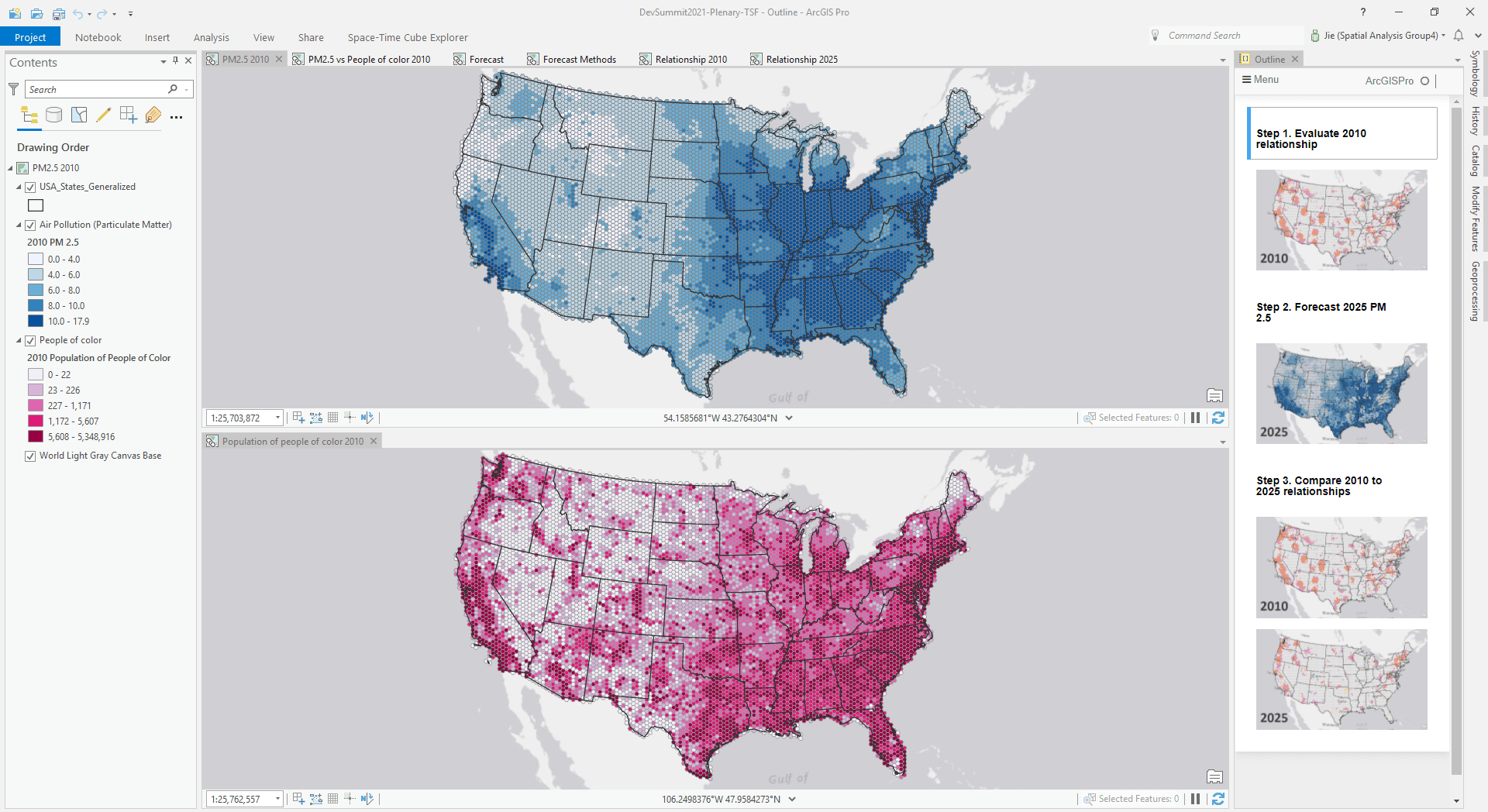
The first goal of our analysis is to find where the relationship between air pollution and the pis strongest. Then, we’ll explore what the future might look like by forecasting our PM 2.5 data to 2025. Finally, we’ll see how the relationship between air pollution and the population of people of color might change in the future. This will help us prioritize action. To do this, we’ll expand on our initial visualization and analysis using machine learning tools in ArcGIS Pro.
The project package is available to download, including a detailed ArcGIS Notebook containing the whole workflow of the analysis.
1. Understand bivariate relationships by local spatial statistics
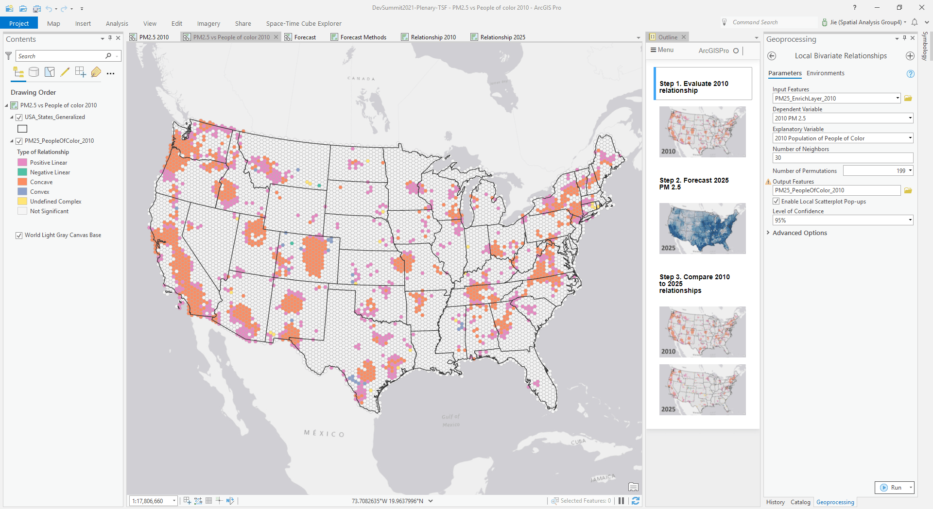
To start, we used the Local Bivariate Relationships tool, a spatial statistic that quantifies where the relationship is strongest and most meaningful. In the below example, the pink and orange colors represent significant positive relationships, meaning, as the population of people of color goes up, so does exposure to air pollution. We can open the automatically generated pop-ups to drill into more information to understand these relationships.
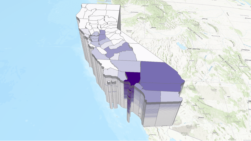
For instance, in the map below (Figure 2), we see an example of a significant positive relationship in California’s central valley. This area is one of the most productive agricultural regions in the nation as well as a place where many migrant farm workers live. Unfortunately, it’s also a place that has been linked to water contamination and to problematic pollution pathways. As such, this area represents inequities that we want to explore and address.
2. Forecast PM 2.5 to 2025
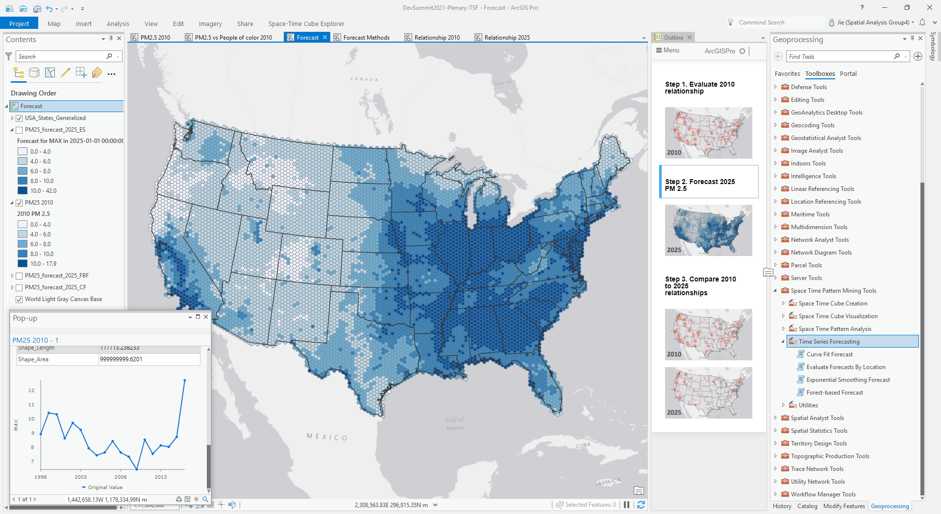
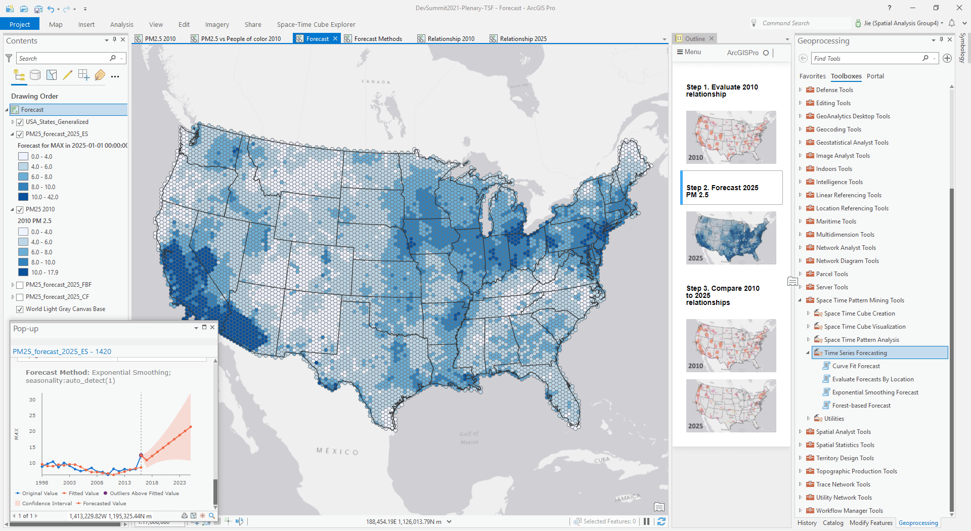
Next, we’ve forecasted the PM 2.5 data to 2025 using the new Time Series Forecasting toolset in ArcGIS Pro. We’ll start with a historical time series at each location from 1998 to 2016 (see Figure 3) to forecast it out to 2025 (see Figure 4).
The toolset provides three ways to forecast:
- The Curve Fit Forecast tool applies a linear, parabolic, exponential, or S-shaped curve to the time series.
- The Exponential Smoothing Forecast tool can incorporate seasonal patterns into the forecasts by decomposing the time series with season and trend.
- The Forest-based Forecast tool uses a machine learning approach to train and forecast the time series with moving time windows.
Figure 4 shows an example of using exponential smoothing on PM 2.5 data. The pop-ups describe our existing data in blue and the fitted and forecasted data in orange. A confidence interval is also provided to better indicate the reliability of our forecast. We can optionally enable outlier detection and see that extremely high outliers are symbolized in purple and extremely low outliers are symbolized in green.
There’s no magic bullet for doing this forecasting across the entire study area, so we want to try each of these approaches to get the best possible predictions. Since the three forecast tools all need similar parameters like input space-time cube, analysis variables, time steps to forecast and exclude for validation, and new options for outlier detection, it’s handy to just define a function in the notebook to run the entire forecasting toolset in sequence.
After applying all three forecasting methods to the data, we can use the Evaluate Forecasts by Location tool to find the optimal forecast at each location. The result is a hybrid prediction where every location is forecasted using the best method, as shown in Figure 5.
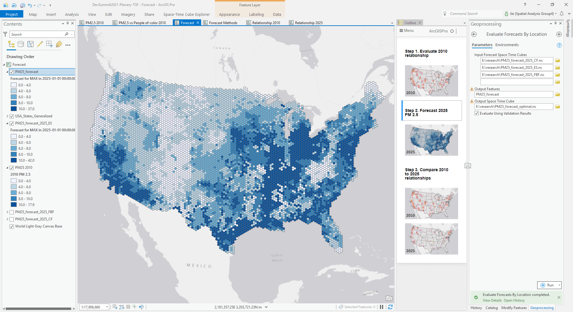
3. Interpret forecast result using a spatial approach
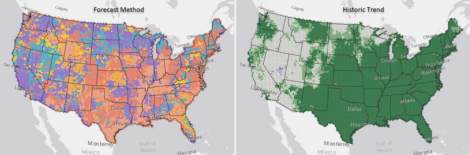
Because we’re taking a spatial approach to this problem and allowing these models to vary from place to place, one of the most powerful ways to understand spatiotemporal patterns is to symbolize the map using the forecast method.
Here’s the fun part. If we put this map side by side with the trend map identified by the Mann-Kendall statistics in Visualize Space Time Cube in 2D tool, as shown in Figure 6, we can see the swath of the country with the significant decreasing trends were mostly in shades of orange, telling that one of the parametric curves could be efficient enough to model the trend. Other locations with no significant trends were detected, predominantly using Forest-Based Forecast or Exponential Smoothing to model the complex time series patterns, like California mainly in purple.
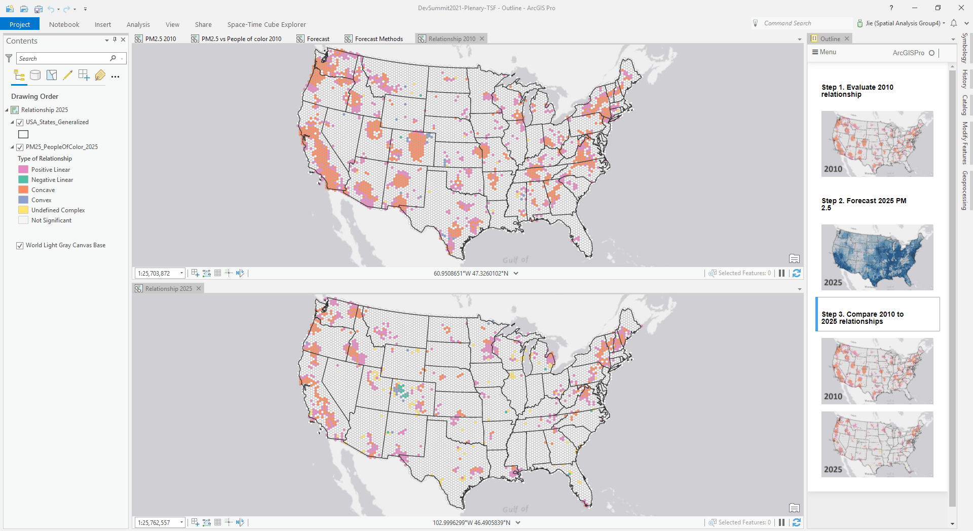
4. Foresee the change of the bivariate relationship in 2025
Finally, we want to see how the relationship between air pollution and the population of people of color changes based on our forecast.
Looking at our local bivariate relationship maps for 2010 on the top and 2025 on the bottom in Figure 7, we see fewer pink and orange areas in 2025, suggesting that we’re moving in the right direction, but there are still inequities and this map shows us where they’re expected to be so that we can prioritize where to take action. And we can use spatial analysis to continue to explore this complex issue for all the communities being disproportionately impacted.
Conclusions
Using the understanding we’ve gained from our spatial approach to forecasting the data, we can see the baseline scenario if no action will be taken. From there, we can guide policy based on unique characteristics of the spatiotemporal patterns of air pollution and prioritize our mitigation strategy. Combining these visualizations and analysis, we can make environmental justice data understandable, forecastable, and most importantly, actionable.
Using ArcGIS Pro as our spatial data science workstation, and the new spatial approaches that we’ve built into the Time Series Forecasting tools, we can solve complex problems across both space and time.


Article Discussion: