For the Spline with Barriers interpolation tool, the enhancements that were made when the tool was implemented in ArcGIS Pro 2.0 are now also available in ArcGIS 10.6. Let’s have a look at the history of this tool, and some example applications.
Tool History
The Spline with Barriers tool was first implemented in ArcGIS more than ten years ago. It was included in the Spatial Analyst and 3D Analyst toolboxes initially as a script tool which called a Java library that performed the interpolation. The tool was not included in the initial release of ArcGIS Pro. However, for ArcGIS Pro 2.0 the tool was rewritten in C++ with some optimizations and bug fixes. This improved C++ implementation is now also available in ArcGIS 10.6, and has replaced the older Java implementation.
Applications
Often we have a variable that is spatially not continuous and we want to use interpolation to produce an output raster that has values everywhere. For example, soil characteristics, or water quality in a braided meandering stream. In these cases you can use Spline with Barriers and specify either a polygon or polyline feature class to define the boundary of the discontinuity.
Methods and comparisons
Spatial Analyst and 3D Analyst have two interpolation methods that have an optional barrier input, those being IDW and Spline with Barriers.
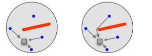
The main difference between IDW and Spline with Barriers, other than the algorithm, is the way in which the points that are to be used in the interpolation are defined. IDW uses a “line of sight” approach, which means that if a point can’t be “seen” because of a barrier, then it is not used to make the prediction at that particular location. Spline with Barriers, on the other hand, weights the points based on the shortest distance around a barrier. In the illustration below, IDW (on the left) will only use 3 points to make a prediction when a barrier intervenes. In contrast, Spline with Barriers will utilize all 4 points to make the prediction.

Case Study
As an example, we’ll use the same case study described in Creating Faulted Geologic Surfaces with ArcGIS by Mike Price in the ArcUser Summer 2014 issue. In this article, the Spline with Barriers tool (the original Java version) is used.
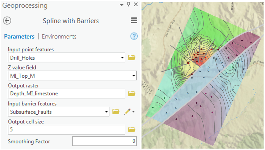
We’ll use the point feature class, which contains the depth to the top of the Mississippian Leadville Limestone, and a polyline feature class defining the subsurface faults, to create an output depth raster with a cell size of 5 meters.


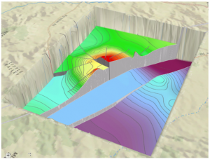
We often rely on contour lines to aid our interpretation of an interpolated surface. However, in the vicinity of fault lines there may be abrupt changes in the depth values between some adjacent raster cells. As a result, we cannot use the standard Contour tool as it will incorrectly produce many contours in these areas. The Contour with Barriers tool is well suited for this type of data as illustrated in the images above.
Conclusion
This exercise shows how to model the elevation of the top of the Mississippian limestone in Lisbon Valley, Utah, using only formation top elevations and fault barriers to generate a reliable predictive elevation surface.

Article Discussion: