Making cool contours with reprojected elevation rasters
This tutorial takes a raster reprojected in the previous article and uses it to create a hillshade, model a slope, and create high-quality contours using a reprojected elevation raster.
In “Looking Good: Properly reprojecting elevation rasters,” an article in the fall 2013 issue of ArcUser magazine, I presented several methods for effectively reprojecting elevation and other rasters using the Nearest Neighbor technique, bilinear resampling, and cubic convolution. That exercise showed how to reproject a digital elevation model (DEM) from geographic to projected coordinates.
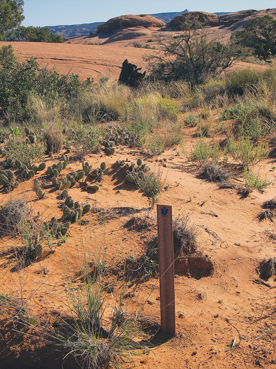
In this exercise, you will generate three related products: a hillshade, a slope raster, and high-quality contours. The hillshade and slope will help assess the quality of the raster by revealing herringbone patterns, tile seams, or other unnatural artifacts in the raster. In addition, slope rasters can be used to evaluate travel impedance when modeling search and rescue response. After evaluating the reprojected DEM, it will be used to generate contours.
Getting Started
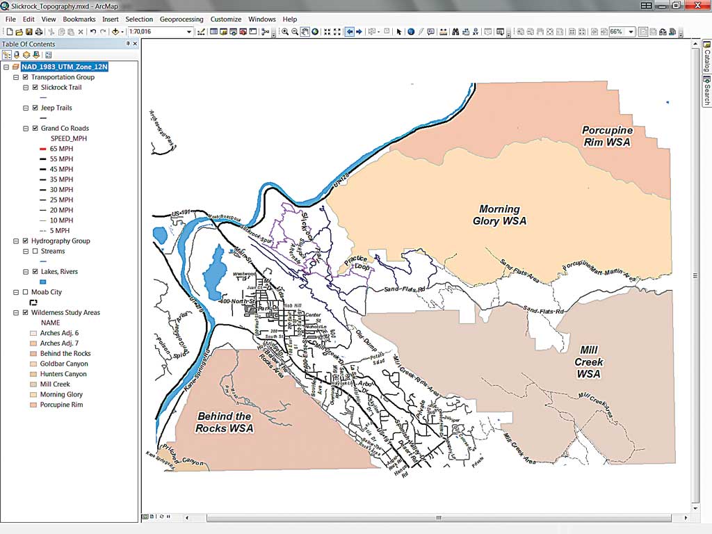
Like the previous article, this exercise uses a small piece of a US Geological Survey 10-meter DEM that shows the famous Slickrock Bike Trail, located just outside Moab, Utah. Download the sample dataset [ZIP] and unzip it on a local drive. Start ArcGIS for Desktop and open Slickrock_Topography.mxd (located in the \Slickrock_Topography folder) in ArcMap. The map includes the Slickrock trail, several jeep trails, Grand County roads, and Wilderness Study Area boundaries. Much of this vector data is available on the Utah Automated Geographic Reference System (AGRC) site.
Setting Up the Model
- In the text menu area, choose Customize > Extensions and enable the Spatial Analyst extension. Choose File > Map Document Properties and set the Default Geodatabase to \Slickrock_Topography\Geodatabase\ UTM83Z12\SR_Topography.gdb. This step is very important if you have completed the previous exercise.
- Still in the Map Document Properties dialog box, check Pathnames Store relative paths, and complete other fields to provide metadata for the map. Click OK and save the project.
- Next, add the reprojected elevation raster by clicking the Add Data button, navigating to \Slickrock_Topography\Geodatabase\ UTM83Z12\SR_Topography.gdb. Add topo_10_utmc. This is an expanded version of the 10-meter topography raster that was reprojected in the previous exercise from geographic coordinates to UTM Zone 12N using the North American Datum of 1983 (NAD83) datum. After careful comparison of the results of the bilinear and cubic resampling techniques, the cubic technique works best in the highly irregular Slickrock terrain. The “c” in the file name indicates cubic resampling was used to reproject this DEM.
- Topo_10 should load at the bottom of the Table of Contents (TOC), and it shows the full extent of the model’s area. To view the entire model area, choose Bookmarks > Slickrock Topography 1:60,000.
- Add ArcToolbox to the ArcMap window and locate the Spatial Analyst Tools. Open the Surface toolset and inspect it.
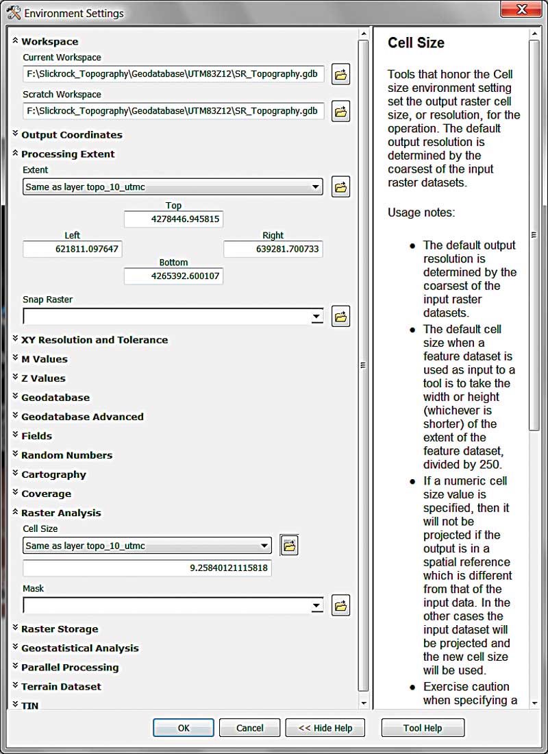
Before using any tools, update the Geoprocessing Environment. These settings are very important. Right-click in an open Toolbox area and select Environments. In the Environment Settings window, verify that the Current and Scratch workspaces are set to SR_Topography.gdb. (This setting should have been carried over from the Map Document Properties dialog box.)
Scroll down the Environment Settings dialog box and set the Processing Extent to Same as topo_10_utmc. Continue scrolling, open Raster Analysis, and set the Cell Size to Same as layer topo_10_utmc. Click OK and save the project.
Modeling the Hillshade
The first task will be to create a hillshade of the DEM.
- Select the Hillshade tool from the Spatial Analyst Surface toolset.
- In the tool’s dialog box, choose topo_10_utmc, located in the SR_Topography geodatabase, as the Input raster.
- Name the Output raster hlsh_10_utmc and save it to the SR_Topography geodatabase.
- Since the elevation horizontal and vertical units for this raster are in meters, a Z factor of 1 is appropriate.
- Accept the Hillshade tool default parameters and click OK. The hillshade layer will appear near the bottom of the TOC.
Organizing the Map
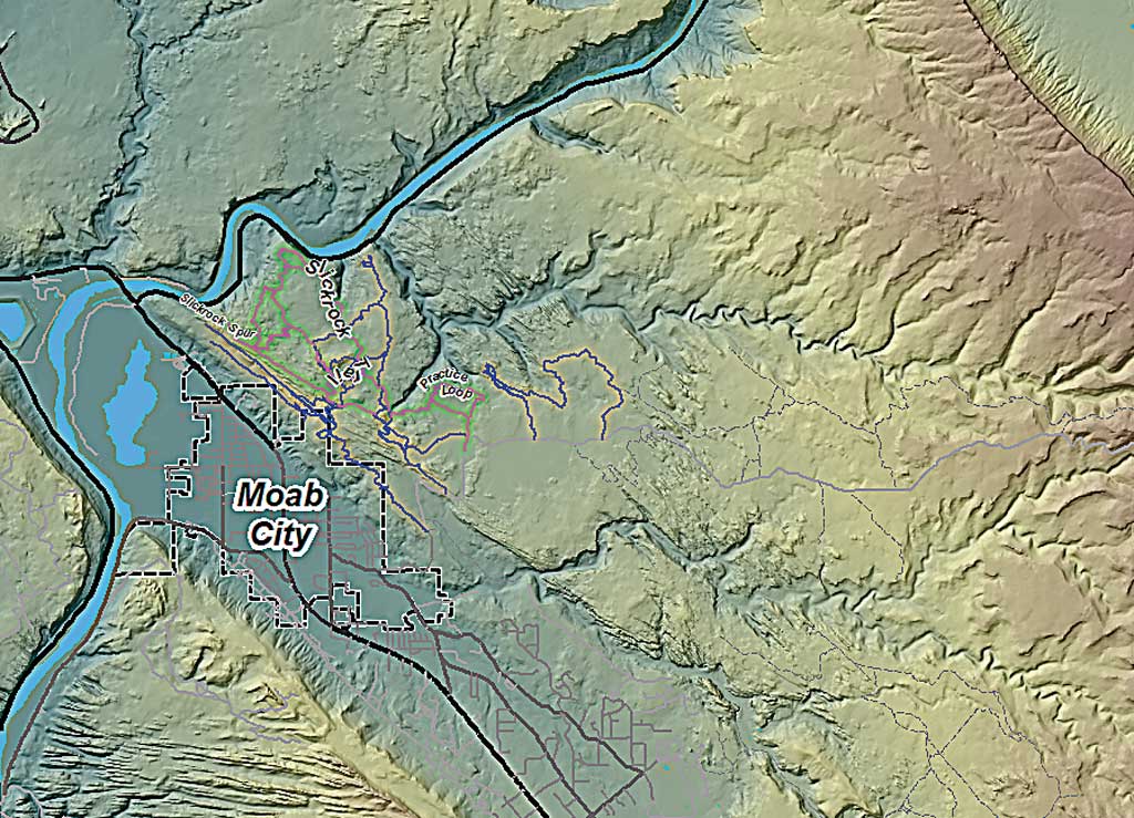
To enhance and organize the map, move topo_10_utmc to the bottom of the layers in the TOC, just below hlsh_10_utmc.
In the TOC, open the Properties for hlsh_10_utmc, select the Display tab, and set Transparency to 50 percent.
Open the Properties for topo_10_utmc. On the Symbology tab, right-click the current color ramp and click Graphic View to uncheck it. This will turn off the color bar and show the names of color ramps instead. Scroll down the list of color ramps and select Brown to Blue Green Diverging, Bright. Also check the Invert box and click OK.
Turn off the Wilderness Study Areas layer.
Investigating Irregular Topographic Slope
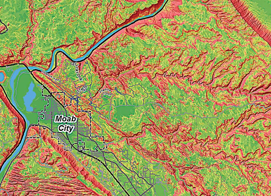
Next, model Slickrock slope to see the ruggedness of this country. Since mountain bikers must battle gravity to go up (and down) the Slickrock trail, modeling the slope in percent will help visualize the effort required to climb these hills. Remember that percent slope is essentially rise over run. In this model, a slope of 10 represents 10 meters of rise for every 100 meters traveled horizontally.
- In the Surface toolset, open the Slope tool and set the Input raster to topo_10_utmc. Change the Output measurement to PERCENT RISE. Name the Output raster slpp_10_utmc (p for percent). A Z factor of 1 is again appropriate. Click OK to the model slope.
- After slpp_10_utmc loads in the TOC, move it to a position just below hlsh_10_utmc. Turn off topo_10_utmc.
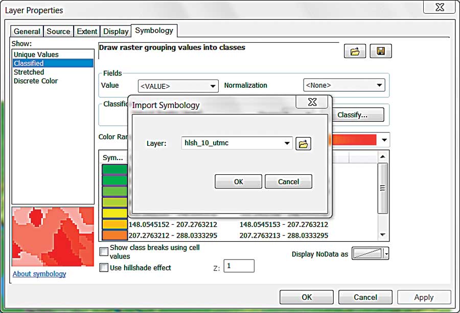
- In the TOC, right-click slpp_10_utmc and open the Symbology tab. In the upper right corner of the Layer Properties window, click the Import (file folder) button and navigate to \Slickrock_Topography\Utility. Select Slope Percent.lyr, a layer file that will apply a standardized classified legend for the percent slope raster. Click Add, then OK, and OK again.
- In the TOC, open the Properties for slpp_10_utmc and select the Display tab, and set Transparency to 50 percent.
- If the legend does not load, check Show and verify that it is set to Classified.
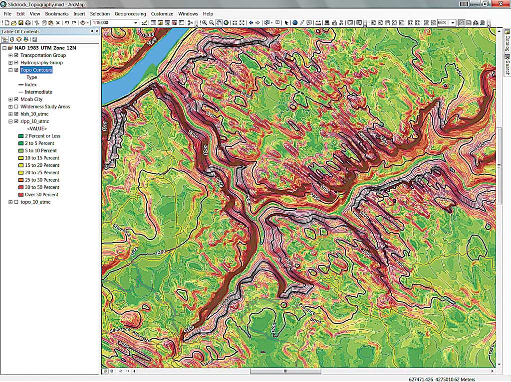
- Use the Slickrock Detail bookmark to zoom in and study relationships between bike trails, jeep trails, and slope. If you have biked in rugged terrain, you will recognized that slopes below 10 percent, shown in shades of green, are usually not too difficult to navigate and that slopes between 10 and 20 percent (yellow shades) are tough. Slopes over 20 percent (shades of red) are typically very dangerous. Fortunately, most of the trails are on green slopes.
- Find a few trail segments that traverse steeper terrain. Notice that the Slickrock Trail is sometimes steeper than the jeep trails, especially in northern areas. These are the slopes I use to set network impedance and calculate travel times when modeling time-based travel on these trails. When finished, save the project.
Creating Contours
The final task will be creating, mapping, and labeling topographic contours. The 10-meter DEM in the sample dataset is of sufficient quality to create contours using a 10-meter interval. Mapping one index contour for every five stacked contour lines will generate an index interval of 50 meters. Wouldn’t it be nice if ArcGIS would flag these 50-meter lines for us? Actually, the Contour With Barriers tool will do just that.
The Contour With Barriers tool has been around for a while but is often underutilized. Initially, it was used primarily by geologists to contour structural surfaces dissected by faulting. Contour With Barriers is now the primary contouring utility for ArcGIS that often replaces both the Contour and Contour List tools.
Displaying Contours
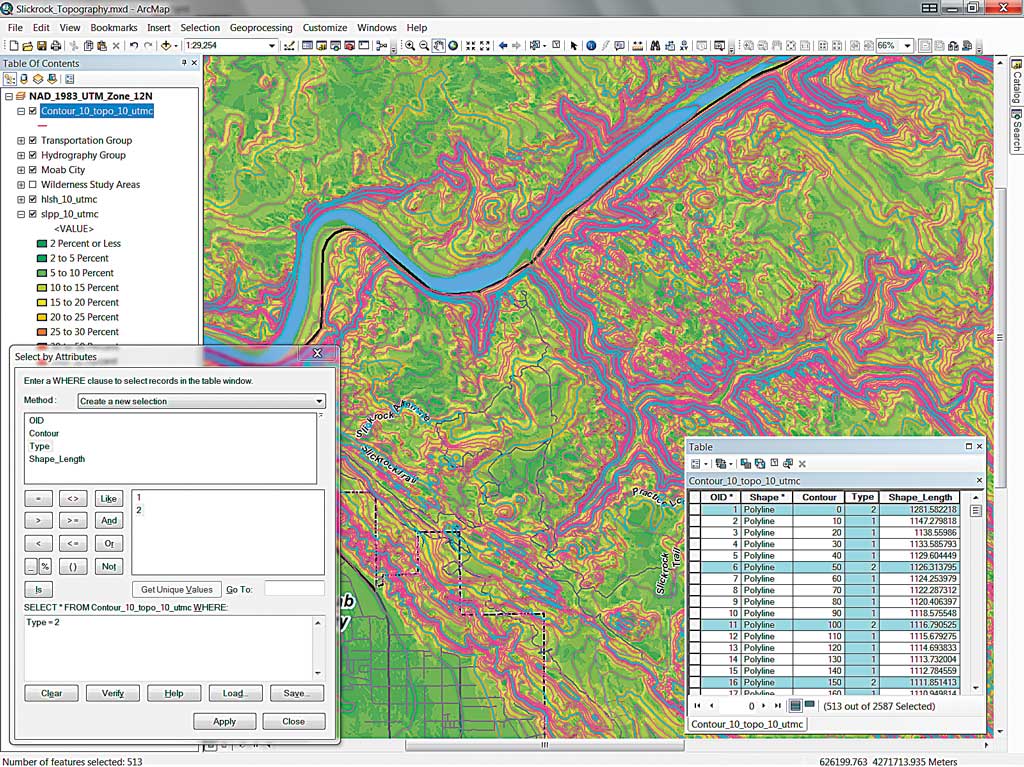
The Contour With Barriers tool adds the Type field and codes index contours with a value of 2. Intermediate contours are coded 1. To simplify thematic mapping and labeling of contours, the sample dataset contains a layer file for symbolizing the contours.
- Open the attribute table for Contour_topo_10_utnc and locate the Type field. Use Select by Attribute to select all records for which Type = 2.
- Click the Add Data button, navigate to \Utility, and select Topographic Contours.lyr. When the layer file loads, note that the data link is broken. You will repair this link by pointing the layer file to Contours_topo_10_utmc file.
- In the TOC, open Properties for Topographic Contours.lyr, click the Source tab, and click the Set Data Source button and navigate to Contour_topo_10_utmc as the data source.
- Remove Contour_topo_10 from the TOC and save again. Cool contours, and they were so easy.
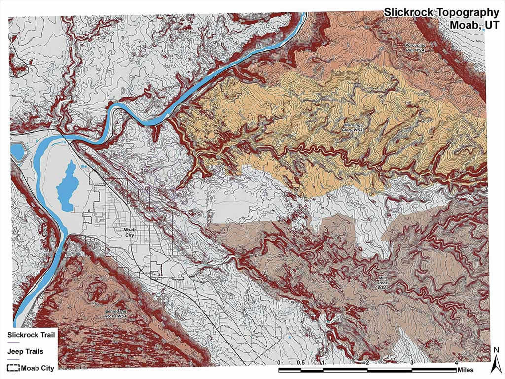
Mapping Contours
Finally, make a presentation map from these rasters.
- Close ArcToolbox to increase the active mapping area and zoom to Bookmark Slickrock Topography 1:60,000.
- Open the Properties for data frame name, click on the General tab, and set the Reference Scale to 1:20,000. Rename hlsh_10_utmc to Hillshade, 10 M Topo; slpp_10_utmc to Slope 10 M Topo; and topo_10_utmc to 10 M Topo.
- Switch to Layout View and look over the map. Turn Slope and Topo layers off; move Hillshade, 10 M Topo above the Wilderness Areas layer; and turn Wilderness Areas back on.
Experiment with zoom scale, reference scale, and label fonts to make the map more attractive and readable. Save once more. You are finished.
Summary
In this exercise, you modeled a reprojected Slickrock DEM and created a topographic hillshade, modeled the slope in percent, and created and posted high-quality topographic contours.
Acknowledgments
The exercise data was obtained from the US National Map and the Utah AGRC, Grand County. I also used files from personal field studies. Esri Spatial Analyst product managers also provided input regarding design and use of tools, especially Contour With Barriers.
