Some of the oldest written records of humans managing infrastructure date back to Mesopotamia, and while our modern systems are more likely to use computers than cuneiform to describe these systems, they both provide methods to record the locations and characteristics of our infrastructure.
The modern solution for managing this information is to store this information in a GIS, and one of the most robust ways of modeling the complex network of manmade infrastructure is to use the ArcGIS Utility Network. This article is intended to act as a bridge, introducing existing GIS users and stormwater subject matter experts to the industry-agnostic terminology and concepts used to describe the utility network to help them better navigate discussions within the utility network community and the online help.
A stormwater utility network is a fully 3D network that includes a predefined set of tables, fields, and rules that can be used to provide an accurate model of your infrastructure. No one’s data is perfect, but the utility network will continuously track your edits, allowing you to validate, review, and correct any issues that arise. The examples in this article are based on the sample model and data included in the Stormwater Utility Network Foundation from Esri.
Modeling Data
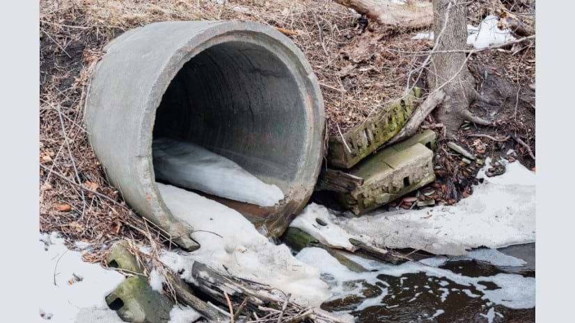
Before you can analyze stormwater data you first need to understand how it is organized in the natural world, and how humans create infrastructure that interfaces with these natural structures. The highest-level structure for organizing surface water capture is a water catchment. This describes an area where rainfall and runoff collect and can enter groundwater or surface water. As we look at how to use GIS to manage these datasets, we should keep in mind that one of our goals is to model the journey of water as it passes through our systems and back into these catchments.

When creating and managing infrastructure it is important to keep these catchments in mind so that we can think of the human made interfaces to these systems as sub-catchments. These manmade interfaces tend to cover much smaller areas than catchments. Where a catchment may describe the area surrounding a lake, the stormwater infrastructure in a nearby neighborhood which routes water to a detention area for filtration is acting as a sub-catchment.
By treating this infrastructure as part of the natural process we must not only consider whether the systems are adequately sized to accommodate the amount of natural and manmade water, but also how the paths that water take through the sub-catchment impact the water quality once it leaves human infrastructure and enters the natural world. Now that we’ve looked at the concepts behind stormwater modeling, let’s discuss how to use the utility network to manage stormwater data.

The utility network is a generic framework designed to support modeling infrastructure from many industries. Because of this, care was taken during its development to use generic, non-industry specific terminology to describe the different components of the framework. Let’s look at some of the basic terminology used to describe the basic building blocks of this framework.
- Utility Network – An object in a geodatabase that contains a collection of classes that provide advanced visualization, editing, and analytical capabilities.
- Domain Network – An industry-specific collection of feature classes and nonspatial objects used to represent the systems important to that industry. Each utility network contains one or more domain networks. Every utility network also contains a special structure domain.
- Network Classes – Each domain network consists of five feature classes and two tables: Device, Line, Junction, Assembly, SubnetLine, JunctionObject, and EdgeObject. You can learn more about the purpose of each of these classes by reading the Classes in a domain network topic in the online help.
- Asset Group – The first level of classification for every feature in the utility network is the asset group. These correspond to subtypes in the data model and control which fields are visible/required for that feature along with the pick lists/domains associated with those fields.
- Asset Type – The second level of classification for every feature in the utility network is the asset type. The rules, editing behaviors, and other utility network configurations for features are almost all based on a feature’s asset type.
These descriptions are adapted from the utility network vocabulary page of the online help, if you are new to the utility network you should consider bookmarking and referring to this page when you encounter an unfamiliar term.

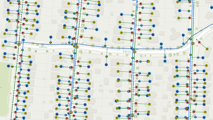
Let’s put this terminology to use and do a quick review of an example stormwater utility network. The utility network is in the same feature dataset as the rest of our network classes. This utility network contains a structure domain network (all utility networks do) along with a stormwater domain network.

Each domain network has the standard set of classes, each of these classes has its own set of subtypes. Subtypes are synonymous with asset groups in the utility network, so each of these subtypes corresponds to an asset group in the stormwater domain network. Looking at the Stormwater Device class, we can see that it has a number of subtypes unique to the stormwater domain.

If we look at one of these asset groups using the Domains view, we can see that it has an asset type field with an asset type domain associated with it representing all its asset types. Below we can see the asset types associated with the outlet asset group of the stormwater device class.

You can review the entire list of asset groups and asset types for the utility network by right-clicking it and selecting the network properties. The resulting dialog shows all the rules and configurations associated with that utility network. The screenshot below shows an example of some of the stormwater device asset types included in the Stormwater Utility Network Foundation.

You can learn more about, and gain access to, the sample industry data models that Esri provides by reading this article about utility network foundations. Now that you understand the basics of how the geodatabase organizes and describes data in the utility network, let’s look at how the utility network applies these concepts to manage connectivity and perform analysis.
Modeling Connectivity
In the previous section we learned that all features for the stormwater system belong to a domain network and saw how different asset types are defined. The next logical question to ask is how does the utility network know what types of features are allowed to be connected? There is a two-part answer to this question. First, the utility network has rules defining which asset types can connect. Second, when the utility network is built or validated it will look at the spatial coincidence of features, along with any logical connectivity defined for features, to determine which features could be connected. It will then create connectivity for all possible connections which have a rule that makes the connectivity valid. Any possible connections without a rule are not created and will create error features in the utility network.
Let’s walk through this process, step by step, below. First, we will start with an example of several rules that allow devices to connect do different types of features:

Each of these rules allows two different types of features to be connected. In cases where the “from feature” is a point feature and the “to feature” is a line feature, we call this a junction-edge rule. The utility network also allows you to model connectivity between two point features, which we call a junction-junction rule. If you are interested in the other types of rules, you can read the network rules section of the online help, but for now we will look at how these two types of rules control behavior within our stormwater model.
To interpret each rule, you start by looking at the “from class”, “from asset group”, and “from asset type” of the first feature. In each of these rules the “from feature” is some kind of stormwater device. Next, you look at the “to class”, “to asset group”, and “to asset type” to see what kind of feature the “from feature” is allowed to connect.
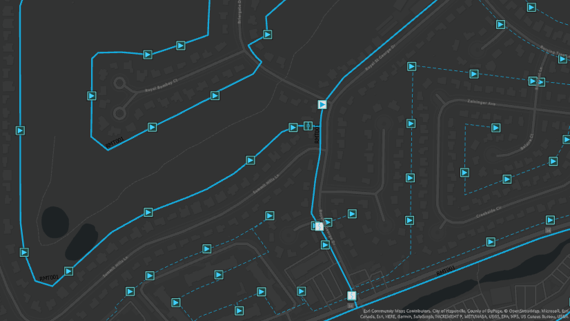
As an example, the first rule in the table above allows a Pipe Inlet (something like a stormwater drain or curb drain) to connect to a gravity pipe. When these features are created and validated by the utility network, it will find this rule and allow these features to be connected. This is very important since these pipe inlets are one of the most common ways for water to enter a stormwater system. You can find a graphic showing each of the four rules below:

Each of these rules is instructive in its own right, but if we combine them, we can see that they allow us to start building out the rule base for a stormwater network. As an example, see the small area below which combines these four rules.

Now that we see how to define valid connectivity, the next question is how do we detect invalid connectivity?
Invalid connectivity occurs whenever there are two features that the system attempts to connect that don’t have a rule. Using the above area as an example, let’s imagine what would happen if we removed the pipe outlet and tried to connect the gravity pipe directly to the open channel using an open channel connection.

The pipe inlet would still be connected to the pipe, and the open channel connection would still be connected to the open channel, because they have rules allowing them to be connected. The gravity pipe and open channel connection; however, would each generate an error due to invalid connectivity because there is no rule that allows them to be connected. This makes sense, because we can’t have a gravity pipe connected directly to an open channel, the water needs to pass through a pipe outlet to enter a channel. The rules we create in the network help us to enforce this.
Each industry data model from Esri includes thousands of rules that define what is allowed to be connected, and these rules give you confidence that your data is properly connected. Because every network edit must be validated, this also gives you confidence that even if you were to have hundreds of versions being edited at the same time, every edit must be validated and therefore every connection is either valid or has an error associated with it.

Conclusion
Now that we’ve covered the basics of utility network terminology, data model, and how connectivity is modeled it’s time to take a moment and reflect on what we have learned. We saw how the utility network gives us a standard set of classes to model each industry, and how these classes were adapted for the stormwater model. We also saw how this data model allows us to configure rules that allow us to accurately capture the details of our stormwater systems. It’s important to remember that all network edits are validated against the rules for the model and these checks, along with any business rules you have configured, giving you confidence that everyone in your organization can trust your data and the results of the analysis they perform.
In our next article we will cover how the utility network uses connectivity to model catchments, and what forms of analysis and validation it provides for these systems. It’s important to remember that because the utility network is supported in mobile, web, and desktop applications everyone in your organization will be able to benefit from access to this data regardless of whether they’re in the office or in the field.
If you have any questions about the utility network, I recommend you visit the ArcGIS Utility Network community site to discuss them with other like-minded professionals. If you want to learn even more about the utility network, you can also read this article about learning resources available for the utility network, including the Learn ArcGIS Utility Network for Water Utilities and Learn ArcGIS Utility Network for Sewer and Stormwater learning series. If you want to download the model and sample data from this article, check out the Stormwater Utility Network Foundation on the ArcGIS Solutions site.
You can also try these hands-on tutorials related to this article:


Commenting is not enabled for this article.