This hands-on blog post, you will learn about the scripting logic and common data workflows that will allow you to get the most out of Python scripting in Insights. You are not a Python user? Fret not! While we will wrangle data using Python in the second half of this post, many of the concepts discussed here can be applied to R as well.
Interacting with scripts
Let’s get to it! Before we dive into our hands-on example, let’s have a look at logic of creating and running scripts in Insights. We will also touch upon certain aspects of the user interface. If you want to familiarize yourself with the entire user interface, check out the official Insights documentation.
Creating scripts
There are two ways to create scripts in Insights:
Creating a new script by opening the scripting environment console: After you selected a Python or R Kernel in the console, Insights will automatically populate the data pane with a script element.
Creating a new script from an existing script: The add to model button in the console toolbar of your existing scripts allows you to create a new script from the selected cell. By doing so, the newly created script gets added to the Insights model. Adding a script to a model is a helpful way to rerun your workflow with different data.
Generally, I recommend limiting the number of independent scripts in your workbook. Insight’s scripting capability is not optimized for many scripts: Each time you open an existing script, the previous Kernel is destroyed and a new one is created. You can reduce scripts by adding multiple functions to one script or by breaking up your code into logical blocks using code cells.
Running scripts
Once you have added your script to Insights and written some code, you have three options to run your script. Each of them serves a different purpose:
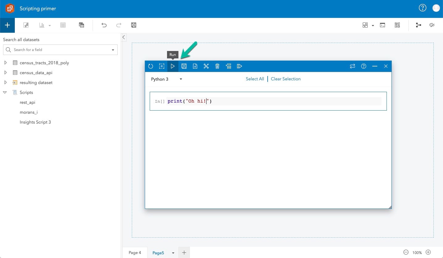
Running in console: Click on the Run button in the scripting environment toolbar. I recommend this method for debugging purposes or if you created a custom Python visualization that you would like to add to your workbook.
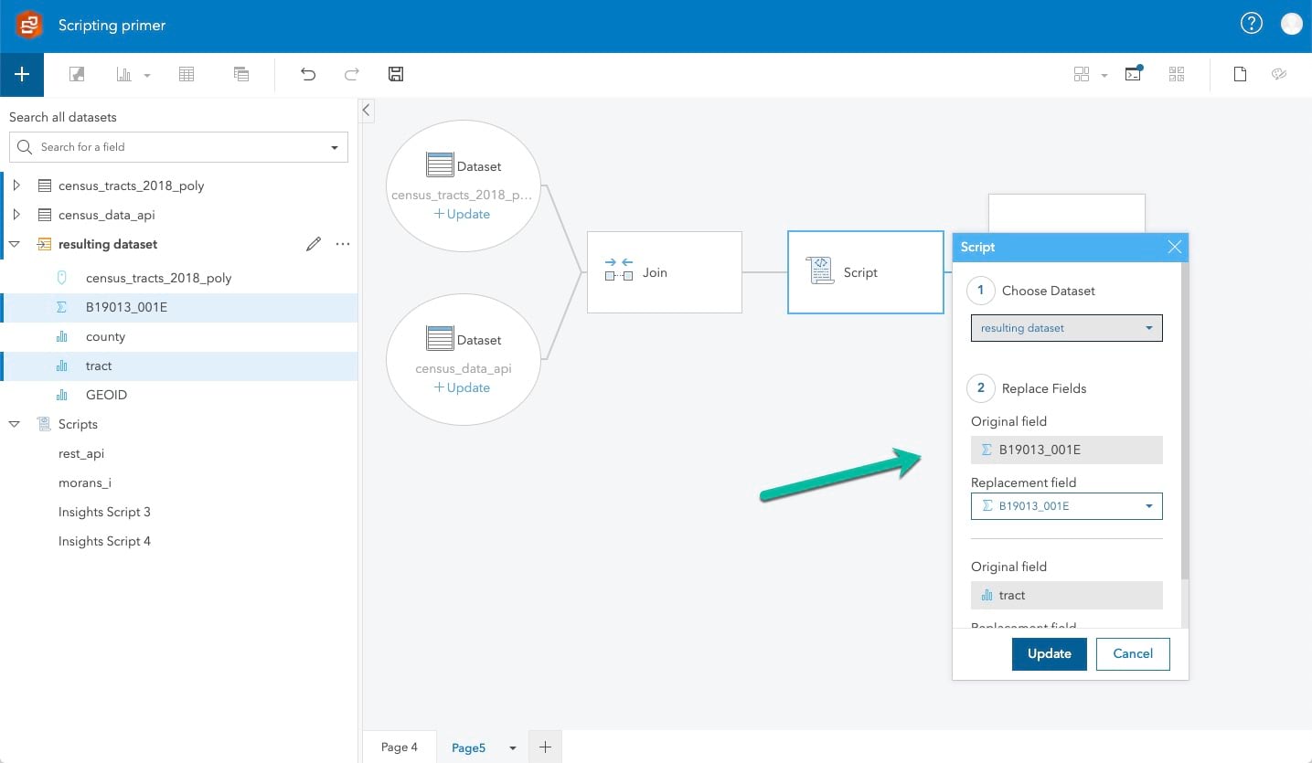
Running from model: In order to run from model, you need to add your script to the model first. In addition, you need to pull in data from Insights into your script (more on this in the second half). Switching to analysis view and clicking on the edit icon will prompt you to replace and rerun the script with new fields. Note: Make sure you rerun your script with valid fields as defined by your script. Otherwise, the script will fail.
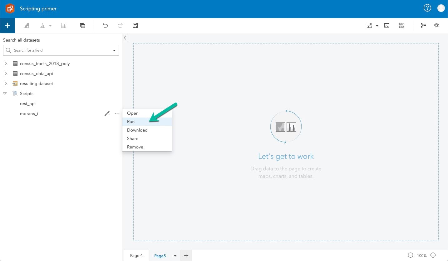
Running from Insights data pane: You can run a script from the data pane by clicking on the three dots to the right of it and selecting run. This will run any script, no matter if it is pulling in data from Insights or not. This is useful if you made a change to your script and want to rerun it without replacing any field names.
Working with scripts: One example, three workflows
Now that we know more about scripting logic, let’s dive into how we can combine scripting with Insights’ core functionalities. I will walk you through three different data wrangling workflows using one example for all three workflows. In the example, we want to find out if there is a spatial correlation between median household incomes of Census tracts in New York City.
Before we get started
We will talk about the general concepts of integrating scripting in Insights and won’t discuss every single line of code. If you would like to see what each line of code is doing, this is what you need to follow along:
- Github repo containing required shapefile and code snippets
- Census API Key
- Kernel gateway to an environment with the required Python dependencies (Documentation on how to setup a Kernel gateway here and list of dependencies here).
- Basic understanding of dataframe structures in Pandas and Geopandas
Workflow one: Querying external data
One powerful scripting workflow is to fetch external data from REST APIs or databases and return it to Insights. This is helpful if your data frequently changes. Instead of updating your own datasource, you can simply rerun the script and pull the updated data. Today, we will use the popular Requests library for Python to fetch median household income data through the Census API. After that, we will format the fetched data using Pandas. To do so, let’s create a new Python script in Insights, rename it to rest_api and import the script from here. Don’t run it yet, we will need to make some changes to the API key first.
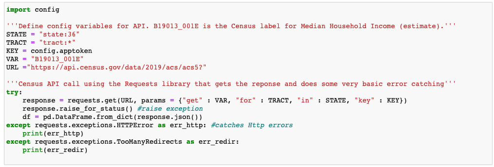
If you are following along, take a minute to examine the code to understand how the API call works. After transforming the API response to a Pandas dataframe and doing some reformatting, we will employ Insights’ magic function to return the dataframe to Insights:
%insights_return(df)
Running the above code will output your dataframe df as a new dataset called layer to the Insights data pane. It is good practice to rename the resulting dataset. Here, we’ll rename layer to census_data_api. Note that there are some limitations to the magic function: It is currently only possible to return Pandas dataframes (no geodataframes or other data formats).
Workflow two: Reading local files
As you might have noticed, the above script imports a script named config on line 1. This is an example of workflow two: storing files locally. You could employ this workflow when you have API keys that you do not want to expose in your workbook. In our example, we created another script named config.py containing a single variable with the API key needed to access our API endpoint:
apptoken = <myapikey>
You need to move this file into a directory named data on the machine where your Kernel gateway is running. The data directory is part of the Kernel gateway directory (It is possible that you have to create the data directory first). From data, your Insights script will be able to access files without you having to specify paths. Now, you should be able to run the above script with your own API key!
Workflow three: Adding datasets to the Insights console
While the above tools are very practical for remote data fetching, let’s walk through at a slightly more involved workflow. Insights comes with many common analysis methods already built-in. But sometimes, you might need a specific statistical method that you cannot find in the core toolkit. Luckily, you can use any library that you can think of with the power of Insights scripting!
Let’s return to our example to demonstrate the last workflow: As mentioned in the beginning, we want to know if there is any spatial correlation between median household incomes of Census tracts in New York City. One way to measure spatial correlation is a statistical method called Moran’s I. Without going into too much detail, Moran’s I is a number that indicates the amount of correlation between spatial features. It is not part of Insight’s core toolkit, but thanks to our scripting interface we can easily run it in Insights. In our case, the spatial features are Census tract polygons.
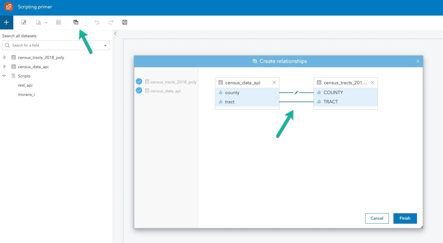
Before we can calculate Moran’s I on them, we need to join our census_data_api data to the polygons. Import the Census tract shapefile into to your workbook and click on the relationship icon in the top left corner. Drag in both datasets into the pane to perform an inner join on the fields COUNTY and TRACT as seen below:
You should end up with a joined dataset. Now, we are ready to make use of another magical Insights trick. First, create a new Python script from console and import the morans_i.py script from the repo. From the joined dataset, drag and drop the fields census_tracts_2018_poly , tract and the field for income, B19013_001E, into your scripting console. In your script, assign them to the variable gdf on line 6. The output should look like this:
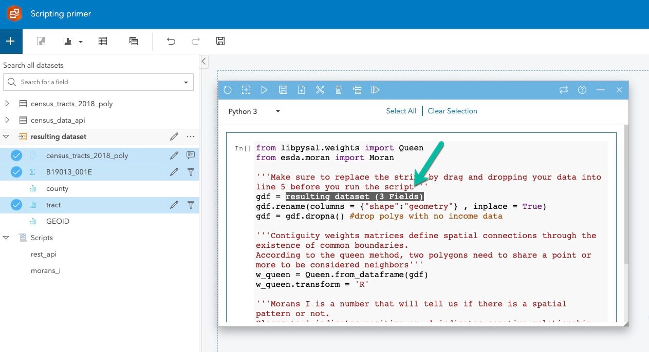
You just created your first geodataframe from an Insights dataset! To verify that this is actually the case, add the code below. It should output geodataframe as type.
type(df)
So what just happened? This behavior is particular to Insights scripting: because it has the Python libraries Pandas, Geopandas, Requests and Numpy baked in, it automatically transforms your fields into dataframes or geodataframes (the latter if your data contains a location field). Similarly, if you want to run other Pandas or Geopandas tools, there is no need to specifically import these libraries. Simply run your tools and append pd, gpd or np as needed.
Now that we have access in our script to the fields required, we are ready to run our script to calculate Moran’s I. We’ll leverage the open-source Python libraries libpysal and esda, which contain all the tools we need. Since they are not part of the Insights scripting setup, these libraries will have to be imported the standard Python way, e.g. by using from libpysal.weights import Queen. Have a look at the entire code before you hit run!
Workflow results
If all went well, you should see a new dataset called layer populate your Insights data pane. Click on the three dots to the right of it and select View data table. You should see two rows, Moran’s I and p-value. We can use this dataset to create a summary table card in the workbook. Congratulations, you made it!

Summary
Let’s rehash the three workflows described above in a more general manner. In workflow one, we looked at a way of using Python scripting to pull in external data, do processing in Python and bring it into Insights for further transformation using %insights_return(<dataframe>).

In workflow two, we imported a local script located in the gateway/data directory on your server machine to pull in information like API keys without having to expose the data in the workbook itself.

Workflow three demonstrated how you can use the drag and drop mechanism to pull in Insights datasets and how they automatically get converted to dataframes or geodataframes. This allows you to run custom Python scripts against Insights data.

What’s next
That’s it for today! If you found this blog helpful, check out our other ArcGIS Insights scripting resources: Learn how to conduct a watershed analysis with Python, check out this blog about Apache Spark and Insights or have a look at our Insights scripting documentation.


Article Discussion: