If you are a data scientist, you probably know about or have used the principal component analysis (PCA) technique, as it is a well-known algorithm in data science. However, I bet you haven’t yet used this technique to analyze a multidimensional raster. ArcGIS Pro 2.9 contains a new principal component analysis tool (named Multidimensional Principal Components tool ) that enriches the capabilities of multidimensional raster analysis in ArcGIS.
Why PCA?
PCA seems sophisticated, and many articles discuss PCA on the web. If you plan to read more without diving into the math, I recommend this blog, as the author explains the complicated algorithm well, using simple language and animated graphs. However, regardless how intricate it is, the primary goal of PCA is simple and clear—data reduction, to transform data into a space of reduced dimension where features and patterns can be easily identified. Image time series data becomes very common nowadays and often difficult to interpret without suitable analytical tools; PCA is a powerful technique for analyzing image time series data and extracting patterns out of it.
Some software packages provide basic APIs for covariance matrix and eigenvector calculation, which are fundamental algorithms of PCA, but to build a real application out of these APIs, you need to invest a substantial amount of time to understand the algorithm, construct data and arrays that are required, decipher the outputs, and visualize the results. It will be even more difficult when it comes to solving the image time series problem. In ArcGIS Pro 2.9, the new Multidimensional Principal Components tool in the Image Analyst toolbox makes it easier. With this tool, you can apply the PCA technique and perform spatial and temporal pattern analysis using image time series data, or a multidimensional raster.
How it works
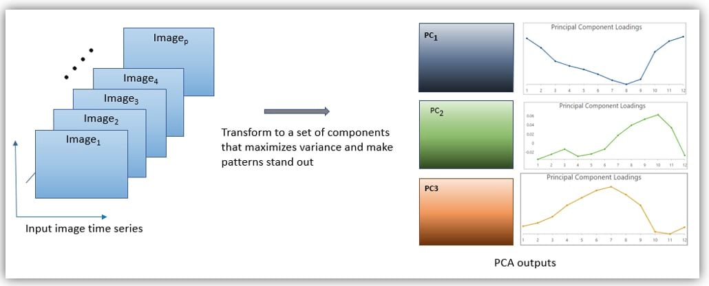
The Multidimensional Principal Components tool takes a multidimensional raster as input—it can be an image time series or image series based on a Z dimension. Behind the scenes, the tool computes a covariance matrix from a series of images, calculates eigenvectors that define a new space in which features and patterns can be revealed better, and transforms the series of images into principal components in the new space. The first component depicts the greatest variation of the input data, and the second component, perpendicular to the first one, represents the second largest variation, and so forth for the rest components.
The tool creates three analysis outputs: an eigenvalue table that allows you to decide how many components you need to keep or drop without losing important information; principal components, stored as a multiband raster, representing the prevalent spatial patterns in the input data; and a loading table indicating the weights each raster contributes to the principal components. The loading chart created from the loading table captures the temporal characteristics of spatial patterns in the principal component raster when the input is an image time series.
You can use the tool directly to obtain the analysis results without having to write a single line of code. Of course, if you prefer Python or Notebooks, arcpy.ia.MultidimesonalPricipalComponents() is the API to use; isn’t that easy?
A case study: Analyze vegetation patterns in Pantanal
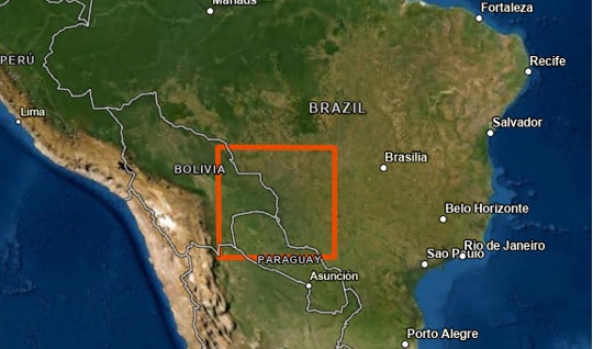
The Pantanal region in South America has the largest tropical wetlands in the world, hosting rivers, lakes, and many kinds of vegetation. Some of the forests and savannas are flooded a few months per year. The unique climate and hydrological cycle from rain (water rising), flood waterfalling, and drought make the vegetation cover quite dynamic throughout the year. A single image of any date cannot capture the variations of the vegetation, and multiple temporal images must be used. So, I am going to use the new Multidimensional Principal Components tool and multiple temporal images to identify the major spatial-temporal patterns of the vegetation cover in this dynamic Pantanal region.
Data preparation
The data used for this study is Enhanced Vegetation Index (EVI) from the MOD13Q1 product. EVI is sensitive to dense vegetation and effective in differentiating types of vegetations in this study area. The temporal resolution of MODIS EVI images is 16 days, but some months might not have qualified images due to cloud and cause gaps. Instead of using data of one particular year, I’ll use data of multiple years.
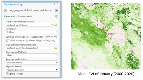
I selected all scenes between 2000 and 2020 with cloud cover less than 10 percent, and then created a multidimensional Cloud Raster Format (CRF); see this video for the detailed steps. I then aggregated the 21 years of data into monthly mean using the Aggregate Multidimensional Raster tool with a recurring monthly keyword. This also reduces the possible noises and NoData pixels in the data. The result from the aggregation operation is a multidimensional raster with 12 slices, each representing the monthly mean across 21 years, and this will be the input for the principal component analysis.
Principal component analysis
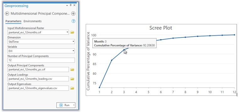
To extract the spatial vegetation pattern, I used the Multidimensional Principal Components tool. The input is a previously calculated monthly EVI time series, set to compute all 12 components, and I’ll let the tool create outputs for me.
The output eigenvalue table contains eigenvalues and cumulative percentages of variance for each of the 12 components. Eigenvalues are ordered numbers, and the first component has the largest eigenvalue. The scree plot (right below) is created using the field of cumulative percentage of variance. You can see that the first three components can explain more than 92 percent of the total variance in the data, and the other nine components only account for less than 8 percent, which we can drop without affecting our analysis result. So, I chose three components to do further analysis.
The map below displays the first component, which is the first band in the principal component raster. The first component extracts an overall seasonal vegetation greenness over the entire hydrological cycle. One thing to note is that principal component raster values are not exact EVI anymore, but they are correlated by the loading values. In the map below, pixels in dark brown denote healthy and leafy vegetation. This can be confirmed by the loading chart (right below). The loadings vary according to the seasons and the hydrological cycle; the high weights from November to March mean the data of these months contributes more to the first component because November to March is the wet season, and forests and crops get higher EVI in this season than July to September, which is the dry season.

The second component picks up the secondary dominant feature. The dark brown pixels in the second principal component raster are related to flooded vegetation. We can confirm this from the loading chart of the second component. Rain starts from October, and the EVI value starts to drop due to the reduction in total leaf area caused by rising water. After December, the EVI decreases from January to May when areas of the flooded vegetation are maximized.

The third component below is associated with grassland savanna. The dark brown pixels in the map are attributed mainly to the data from June to August when flooding retreats and grassland savanna becomes green.

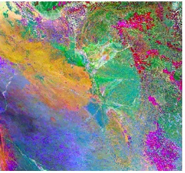
If I display these components using RGB render, in which the red channel is the first component, green is the second component, and blue is the third component, the patterns stand out. Red indicates crops, and orange is forests because these come from the first component. Green is water or flooded vegetation, which is from the second component, and blue is mainly from the grassland. So, the RGB composite map and the associated charts depict the spatial and temporal patterns of the vegetation in the Pantanal region.
Classify PCA result
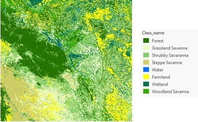
We can go one step further to classify the PCA result. Here I defined eight classes as suggested by Isnard et al. in the article [1] and created this vegetation cover map of the Pantanal region using a support vector machine classifier. Since the focus of this article is on multidimensional PCA, for the detailed steps on the image classification workflow, see this learn lesson.
One special note for this workflow, the RGB display of the principal component raster highlights the different types of the savannas. In addition, with the assistance of the loading chart that characterizes the seasonal pattern and the reference check on the ArcGIS Online basemap, these help collect training samples without visiting the fields.
Summary
The ArcGIS Image Analyst toolbox contains many tools for multidimensional analysis and in particular, image time series analysis. You can perform change detection from an image time series, finding out when pixels have an abrupt change or gradual change in the forest applications; create a predict raster using the Random Forest Regression tool from observations and multidimensional variables; calculate anomaly from multidimensional raster using the Generate Multidimensional Anomaly tool, and you can also model the linear or seasonal trend using the Generate Trend Raster tool. The new Multidimensional Principal Components geoprocessing tool helps uncover features and patterns from image time series that cannot be fitted with a known model.
This blog provides just one example, and you can use this technique on climate data, ocean data, atmospheric data, and more, and create more interesting applications.
In terms of PCA for multidimensional raster, there are two ways to analyze. In this example, we analyze the image series by treating each raster as a member of the time series, looking at the spatial pattern in the data. Another way is to analyze each pixel time series by treating pixel arrays as the member, identifying the temporal patterns that exist in the time series. I will discuss more when this capability is available in a future release.
Reference
[1] Isnard, T; Penatti, N, Ferrira, at el., Principal component analysis applied to a time series of MODIS images: the spatio-temporal variability of the Pantanal wetland, Brazil, February 2015, Wetlands Ecology and Management 23(4):737-748

Article Discussion: