ArcGIS Pro 2.7 introduces a new tool, Surface Parameters, for analyzing the characteristics (slope, aspect, and curvature) of a surface such as an elevation surface or DEM. It is available with either a Spatial Analyst or 3D Analyst license. If you use the existing Slope, Aspect, and Curvature tools, the Surface Parameters tool is your new, better alternative with quite a few improvements. Some of these improvements are useful across most surface analysis metrics so we put them all in a single tool for a consistent experience, which also make it easier for us to add new analysis metrics in the future. This blog introduces the tool and some of its notable improvements.
Surface analysis of high resolution DEMs
Using mathematical and statistical methods to analyze the characteristics of a terrain surface (a field known as geomorphometry) is typically done to quantify and understand the current shape of the landscape and land forming processes. These tools are used to determine the suitability of an area for a particular use such as residential development or agriculture, identify areas as risk for landslides, or find an optimal route through a landscape with no roads. Traditionally algorithms for such analysis used a 3 x 3 moving window of cells, and with DEM cell size typically in the 10 meter to 90 meter range in the past, the 3 x 3 window was appropriate for capturing land surface processes.
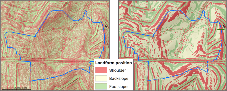
As the resolution of available DEMs becomes finer and finer, the data has become overly detailed for the phenomena we are trying to model. For example, knowing the slope, aspect, or curvature of a 1 meter square of ground to determine if a hectare of land is appropriate for development is typically more detail than we need. A common workaround to this problem has been to resample the DEM to a larger cell size, which takes time and disk space. Resampling can also reduce the fidelity of the data or introduce artifacts. The new Surface Parameters tool contains a Neighborhood Distance parameter that allows you to specify a distance which is appropriate for the phenomena you are trying to model.

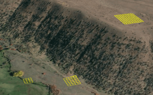
Higher resolution elevation data often contain some undesirable artifacts (errors) as a remnant of the source data collection or processing as illustrated in the graphic above. Using an extended neighborhood helps to minimize the impact of these artifacts. The quadratic surface fitting described below also helps to minimize the impact of such artifacts.
There is also an Adaptive Neighborhood option which evaluates the local variability of the terrain and chooses the largest appropriate neighborhood size for each cell. This can be particularly useful with gradual homogeneous terrain interrupted by streams, roads, or sharp breaks in slope.
No projection distortion
To eliminate distance distortion from the use of projected coordinate systems the new tool performs all internal distance calculations in geodesic space. This is also beneficial since DEMs are often delivered in geographic coordinate systems, and with geodesic calculations there is no need to reproject the DEM or think about a Zfactor.
Improved surface fitting
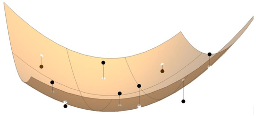
Slope, aspect and curvature calculations all work by fitting a surface to a neighborhood of cells as mentioned above. In the past we’ve used different approaches for different tools but have now unified that approach in the Surface Parameters tool. The Slope and Aspect tools have traditionally fit a plane to those cells, but a plane is rarely a good descriptor of the landscape and may mask natural variations of interest. The Curvature tool traditionally used a biquadratic surface which provides a tight fit to the data and is sensitive to noise and errors common with modern high resolution DEMs.
The new tool uses a quadratic surface by default, which provides a more natural fit to the terrain than a plane, without amplifying noise in the data as biquadratic may be prone to do. Surface Parameters also includes a biquadratic option.
New curvature types
The Surface Parameters tool introduces 3 new types of curvature to ArcGIS and new nomenclature for naming them, adopted from a recent paper by Minár et al., 2020. For those with a particular interest in land surface curvature I highly recommend this paper, which provides a comprehensive review of the history, uses, and prior software implementations, with an effective categorization and naming of the many types of land surface curvature.
The new curvature methods are geometric curvatures, whereas the profile and planform curvature of the Curvature tool are directional derivatives of the surface. Conceptually, geometric curvature finds the best fitting circle (osculating circle) to approximate the shape of the curve at any point, and is computed as the reciprocal of the radius of the circle (1/r). Therefore the flatter the surface, the bigger circle to fit, and smaller the curvature.

The Profile (normal slope line) curvature surface parameter measures the geometric normal curvature along the slope line. Sometimes referred to as “profile curvature”, it can be visualized as the shape of a vertical (profile) cross section through the surface. As illustrated below, the vertical plane cuts through the surface along the orange line, and if cut away would appear as a cross sectional profile of the surface.
That plane is defined by two vectors, the yellow arrow showing gradient direction or slope line arrow, and the red arrow indicating the surface normal. It is the combination of these red and yellow vectors that define the light orange plane and its orange line of intersection with the surface. The profile curvature is computed along the orange line (normal slope line) in the orange plane.
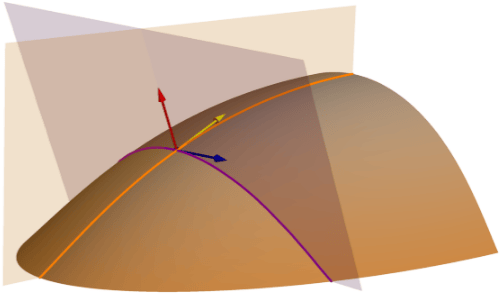
Profile curvature is typically applied to characterize the acceleration and deceleration of flow down the surface by force of gravity. At higher velocity water can carry and move larger amounts of material, therefore areas of acceleration become areas of erosion and areas of deceleration become areas of deposition.
The Tangential (normal contour) curvature surface parameter measures the geometric normal curvature perpendicular to the slope line, tangent to the contour line. It is referred to as the tangential curvature because it measures the curvature tangent to the contour line. Referring back to the graphic above, it is described as “normal contour” because the purple cutting plane which creates the purple line the curvature is computed along, is defined by the blue contour vector and the red surface normal vector. Tangential (normal contour) curvature is typically used to describe topographic convergence and divergence of flow across the surface.
The third new type of curvature is Mean curvature and is computed as the average of the minimum and maximum curvature. It is also mathematically equivalent to the mean of the Profile (normal slope line) and Tangential (normal contour) curvatures.
While thinking of curvature as the size of a circle fitted to the surface and looking at the orange and purple cutting planes in the graphic above, look at the illustration below. Try to imagine the orange and purple planes for profile and tangential curvature cutting through the surface, the line that would create on the surface, and the size of circle that would best fit that line.

Notice the high convex profile curvature in purple (erosion) around the rim of the crater, and high concave profile curvature in orange (deposition) around the base of the cone. On the right notice areas of high concave tangential curvature in red (convergence) inside the crater, and high convex tangential curvature in blue (divergence) on the ridge facing you. Areas with small curvature values are transparent to improve interpretation.
New Aspect option
The Surface Parameters tool also includes Aspect and uses the same neighborhood and surface fitting options. It provides a new option to choose between geodesic and projected geodesic aspect calculations. The projected geodesic option is used when the aspect output will be used as input to the Spatial Analyst distance tools and optimal path tools. This option was also added to the Aspect tool in ArcGIS Desktop 10.8.1.
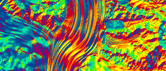
We’ll continue to add new surface analysis methods to the Surface Parameters tool, and be on the look out for future blog posts and articles about these capabilities and their use.
References
James D.E., M.D. Tomer, S.A. Porter. 2014. Trans-scalar landform segmentation from high-resolution digital elevation models. Poster presented at: ESRI Annual Users Conference; July 2014; San Diego, CA.
Minár, J., Evans, I. S., & Jenčo, M. (2020). A comprehensive system of definitions of land surface (topographic) curvatures, with implications for their application in geoscience modelling and prediction. Earth-Science Reviews, 103414. https://doi.org/10.1016/j.earscirev.2020.103414

Article Discussion: