A significant advancement in spatial data analysis in recent years is the integration of space and time for comprehensive multidimensional analysis. Traditionally, density analysis tools were confined to two-dimensional data interpretation, which restricted the capacity to identify complex patterns that unfold over time or across varying elevations. For example, ocean observation includes analyzing time and elevation data to study variations in salinity and temperature at various depths or understand the vertical stratification and circulation patterns of the ocean over time. In this context, the Space Time Kernel Density tool in ArcGIS Pro stands out as a solution, extending traditional 2D density analysis by incorporating a temporal component (t) and an additional spatial dimension using elevation (z). This allows you to investigate trends and patterns within a multidimensional framework.
The Space Time Kernel Density tool can handle three scenarios: with only time (x,y,t), with only elevation (x,y,z), and with both time and elevation (x,y,z,t). This blog article explores how the Space Time Kernel Density tool transforms complex datasets—from decades of storm events to detailed oceanographic and atmospheric measurements—into actionable intelligence. This article will examine the use of time and elevation dimensions in separate analyses. Next, it will explore how combining both these dimensions can unlock richer insights. Finally, it will discuss how to leverage NetCDF and Voxel Layer capabilities using the Scene Viewer, for a more interactive 3D visualization.
Time dimension in Space Time Kernel Density analysis
The Space Time Kernel Density tool extends the classic Kernel Density estimation into the time dimension using the Search Time Window (t) and Time Interval parameters, allowing users to examine how spatial phenomena evolve over time. The Search Time Window (t) (kernel_search_time_window in ArcPy) parameter defines the temporal extent within which events will influence the density calculation. The parameter enables the tool to include events occurring within a specified time range (a few hours, days, or weeks before or after a given time), ensuring that the density estimate reflects both immediate and nearby temporal occurrences. On the other hand, the Time Interval (time_interval in ArcPy) parameter specifies the granularity of the time intervals used in the analysis. It specifies the length of each time interval, such as 1 hour, 1 day, or 1 month. This granularity allows for detailed temporal analysis, such as detecting periodic trends or assessing the impact of climatic cycles over time.
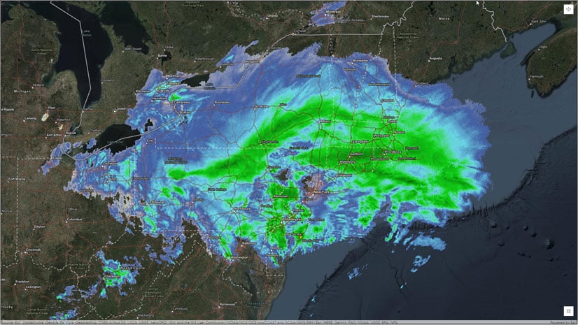
This example uses the NOAA Storm Events Database covering a time period from 1950 to 2020. In this analysis, the kernel density is computed using a 5-year search time window, a 30-day time interval, and a 250-kilometer search radius in the (x,y) dimension. You can further aggregate the output raster at quarterly and yearly intervals using the Aggregate Multidimensional Raster tool. This approach highlights the seasonal patterns and long-term changes in storm frequency. Specifying the parameters–such as a 5-year search time window, a 30-day time interval, and a 250-kilometer search radius–allows for a focused analysis of storm events over a defined timeframe and spatial extent. This helps to capture the density and distribution of storm occurrences, revealing seasonal patterns and trends in frequency over the years. By aggregating the output raster at different intervals (daily, weekly, monthly, quarterly, or yearly), one can gain insights into both short-term fluctuations and long-term changes in storm behavior, enhancing the understanding of climate impacts over time.

Understanding vertical variability
Beyond the time dimension, the Space Time Kernel Density tool allows the integration of elevation data in kernel density estimation. Through this integration, you can analyze any phenomena that vary with depth or height. The tool uses a search radius in the elevation dimension and an elevation interval to enable analysis with elevation data. Similar to the temporal counterpart, the Search Radius (z) (kernel_search_radius_z in ArcPy) parameter allows the user to define a range for analysis in the vertical dimension. This means that the tool examines the data in discrete elevation bands and enables the identification of sharp gradients or subtle shifts in conditions. The Elevation Interval (elevation_interval in ArcPy) parameter defines the size or thickness of each vertical segment included in the analysis. By breaking the vertical dimension into consistent slices based on the set interval, the tool allows you to detect small changes or trends at different heights without the analysis becoming too noisy or too detailed.
This example uses the Global Navy Coastal Ocean Model (Global NCOM) data to explore how temperature varies with depth. The data was analyzed in 10-meter elevation intervals with a 75-kilometer search radius in the (x,y) dimension. This helps to identify changes in temperature at different depths and shows how the water layers are arranged.
")
Integrating time and elevation dimensions
In ocean observations, data is often collected over a specified time across elevation. To understand the density trends at different heights (or depths) over time, it is recommended that you run the Space Time Kernel Density tool with both time and elevation dimensions. Since the output density raster will include time and elevation dimensions, you can use the time and range sliders on display to edit or change visualization. The Range and Time tabs will also be available to customize the output multidimensional density raster.
")
Bringing data to life in 3D: Visualizing with multidimensional voxel layers
By default, the Space Time Kernel Density tool creates a multidimensional raster output in Cloud Raster Format (CRF). You can also select NetCDF as the output raster type. NetCDF is ideal for multidimensional datasets, allowing to retain the structure of time, elevation, and spatial components. If NetCDF is specified as the output raster type, the tool offers to create an optional voxel layer. The voxel layer is created using the output NetCDF file. It represents volumetric data, allowing you to visualize and interact with the data in 3D.
If you run the tool with a voxel layer output or only NetCDF output raster type, there will be no contents added to the Contents pane except when you are on a local scene. There will be a notification stating this. You can use the output NetCDF raster to visualize it in a local scene or use other tools available in ArcGIS Pro such as Describe NetCDF File to understand the output NetCDF raster.

If the Space Time Kernel Density tool is run in a local scene, the tool will create and add a voxel layer to the Contents pane by default. If you only create a NetCDF raster output without creating the voxel layer, you can use the NetCDF raster to add the voxel layer to a local scene using the Add Multidimensional Voxel layer dialog box.
")
Summary and takeaways
Multidimensional analysis capabilities offered by the Space Time Kernel Density tool in ArcGIS Pro provide the opportunity to move beyond the traditional two-dimensional views and extract nuanced insights from complex datasets. Whether you are examining decadal storm patterns, ocean stratification, or climatic changes, the approach of using customizable search windows and intervals in all dimensions allows you to derive insights about complex temporal patterns and vertical variations across defined segments, all while integrating these dimensions seamlessly. The integration of NetCDF and 3D voxel layer visualization further enhances the ability to communicate findings more effectively and in a more appealing way. You can experiment with these features in Space Time Kernel Density tool to unlock new perspectives in your data and explore how they can be tailored to your specific analytical needs. The future of spatial analysis is multidimensional, and ArcGIS Pro is leading the way.
This is the second blog in a series of five blogs, introducing a new approach to understanding density analysis. The Doing more with Density tools: Understanding spatial patterns of data in ArcGIS Pro article demonstrated the similarities and differences among the density tools in ArcGIS Pro and the appropriate usage of density tools to address common issues. The next blog article will discuss performing spatial analysis with density tools in the presence of barriers.
If you are interested in learning more about density tools, see the following conceptual documentation and look for future blog articles focusing on Density tools:
- Understand density analysis
- How Kernel Density works
- How Space Time Kernel Density works
- Difference between point, line, and kernel density
References
- Garcia, H.E., T. P. Boyer, R. A. Locarnini, J. R. Reagan, A. V. Mishonov, O. K. Baranova, C. R. Paver, Z. Wang, C. Bouchard, S. Cross, D. Seidov, D. Dukhovskoy (2024). World Ocean Database 2023: User’s Manual. A.V. Mishonov, Technical Ed., NOAA Atlas NESDIS 98, pp 129., http://doi.org/10.25923/j8gq-ee82
- Martin, P. J., Barron, C. N., Smedstad, L. F., Campbell, T. J., Wallcraft, A. J., Rhodes, R. C., … & Carroll, S. N. (2009). User’s manual for the Navy Coastal Ocean Model (NCOM) version 4.0. Ocean Dynamics and Prediction Branch, Oceanography Division, Naval Research Laboratory, Stennis Space Center, MS. NRL/MR/7320-09-9151. https://www.ncei.noaa.gov/products/weather-climate-models/global-navy-coastal-ocean
- NOAA / National Centers for Environmental Information, (2024). Storm Events Database. https://www.ncdc.noaa.gov/stormevents/

Article Discussion: