Density analysis is one of the fundamental concepts of any geospatial system, and it is used in various contexts to understand the clustering of events at multiple locations. While many choices are available for density analysis in the ArcGIS suite, the Space Time Kernel Density tool in ArcGIS Pro 3.2 captures the temporal patterns in addition to the existing capabilities. You can use tools like Kernel Density or Point Density to understand the distribution of incidents or occurrences in space differently. Since there are similarities between the density analysis tools and their functionalities, it is important to understand which tool you need, how the data is spatially distributed, how spatial and temporal patterns are clustered, and how to use the appropriate tool for analysis.
Analysis tools
Consider an example with a real-world application scenario. In this scenario, to understand the spatial distribution of crime incidents within a city, the police department or the city council may want to carefully examine the spatial distribution and clustering of incidents over time. It might be beneficial to examine the spatial distribution and clustering of the 311 calls during the same time period to see any possible correlation between the incidents and calls.

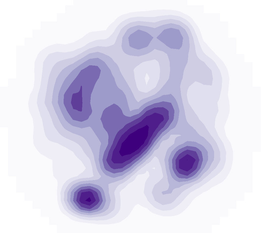
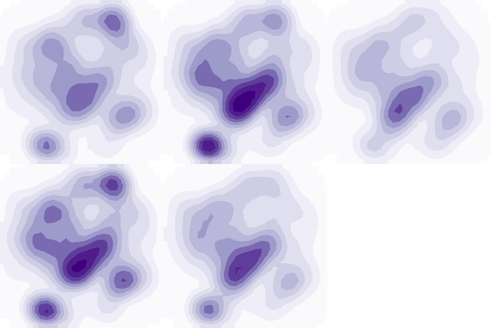
Conceptual figure displaying incident locations (left), traditional kernel density (middle), and kernel density over time (right)
One approach to understanding the spatial distribution of the crime incidents and clustering would be to look at the number of incidents within a defined area (magnitude per unit area). ArcGIS offers multiple tool options to perform this spatial analysis. The Point Density, Kernel Density, and Space Time Kernel Density tools in the Spatial Analyst toolbox can be used for this purpose.
The Point Density tool will calculate the density of point features around each output raster cell. It assumes uniform weights for each point irrespective of the distances between the two points. Conceptually, a neighborhood is defined around each raster cell center, and the number of points that fall within the neighborhood is totaled and divided by the area of the neighborhood. The point density output rasters for the reported crime incidents and 311 calls indicate a prevailing cluster around the downtown area. While the crime incidents density map also has other clusters, for the 311 calls map, the region between South End and Downtown appears to be the hotspot. However, since the Point Density tool only considers the incidents within the unit area, the distance between individual incidents does not have any effect on the output raster.
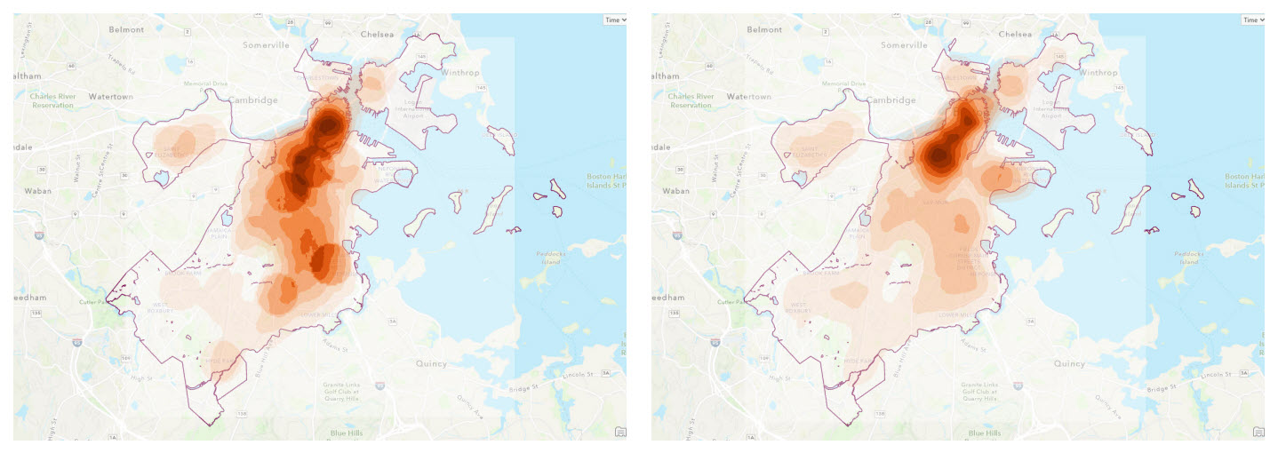
To consider the effects of distance between the incident locations on the density calculation, you can use the Kernel Density tool.
By considering the (weighted or unweighted) distance between incidents, the Kernel Density tool provides a different insight into the clustering of the incidents compared to the traditional Point Density tool. This is because there is a difference between how the two density tools calculate density and consider the radius around the incident points.
In contrast to the Point Density tool, the Kernel Density tool calculates a magnitude-per-unit area from point or polyline features using a kernel function to fit a smoothly tapered surface to each point or polyline. Conceptually, a smoothly curved surface is fitted over each point. The surface value is highest at the location of the point and diminishes with increasing distance from the point, reaching zero at the Search radius distance from the point. While the Point Density tool supports four types of neighborhoods (Rectangle, Circle, Annulus, Wedge), the Kernel Density tool only supports a circular neighborhood. Although both the outputs display the concentration of points in some areas, the output raster created by the Kernel Density tool is smooth due to the use of the kernel function. The Point Density tool is more useful for equally contributed occurrences in which the distance between two points is not weighted (such as Facility locations and counts).
Understanding the temporal distribution
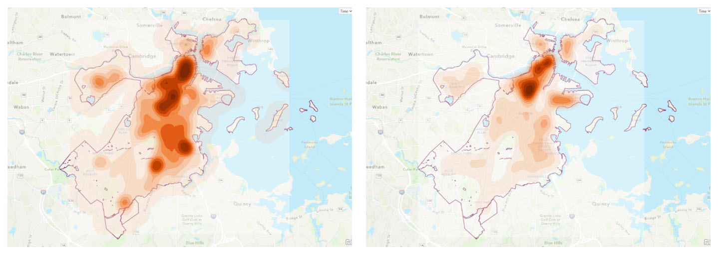
While the output from both these tools offers insight into the spatial distribution and clustering of the incidents, any insights into the distribution of these occurrences over time is still missing. You can split the temporal data and run the tools for individual years and use those for the information; however, that is not always the most efficient approach or solution. The Space Time Kernel Density tool allows you to calculate density considering both time and elevation. In this case, to understand the density of crime incidents in Boston over time, you can employ the Space Time Kernel Density tool to understand the spatial distribution of the incidents while also gaining insights into their temporal distribution and clustering patterns. The output from the Space Time Kernel Density tool is a multidimensional raster, either in Esri’s Cloud Raster Format (.crf) or as a NetCDF (.nc) file. It will contain slices based on the defined intervals.
This example used a one-year time interval to understand the yearly distribution between June 2015 and June 2023. Therefore, the output CRF raster has eight dimensional slices. If you use the Aggregate Multidimensional Raster tool to create an aggregated density raster for all the slices together, it will give you an idea of the overall distribution. The advantage of using the Space Time Kernel Density tool is that it offers to define the search radius in all dimensions (x, y, z, or t).

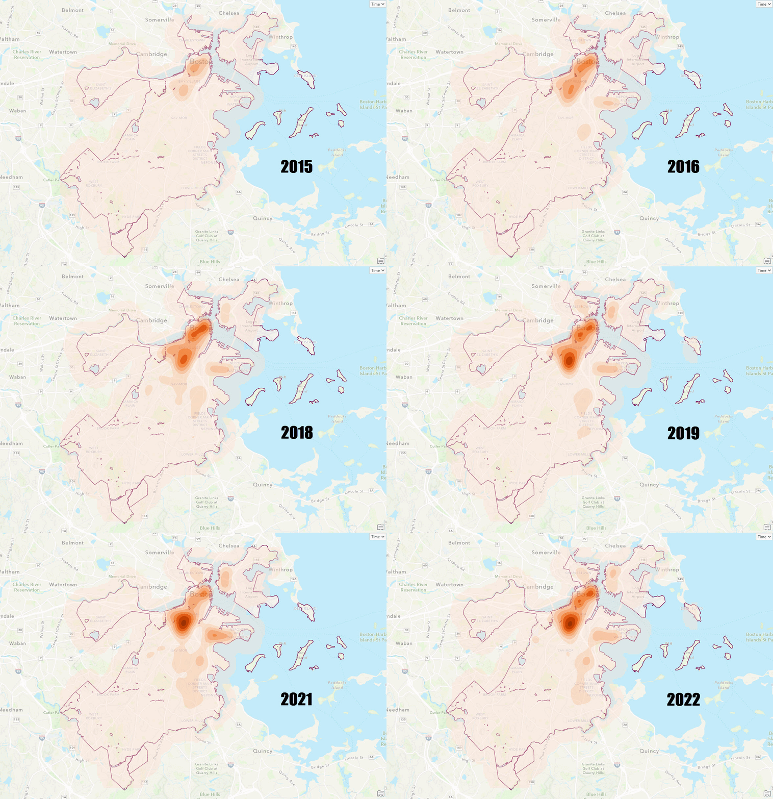
Density map of crime incidents (left) and 311 calls (right) in Boston using the Space Time Kernel Density tool
The Space Time Kernel Density tool allows you to use other multidimensional tools to better understand the density distribution. For example, with the density raster calculated using the Space Time Kernel Density tool, you can identify the temporal trends using the Predict Using Trend Raster tool or create a Dimension profile chart to understand the distribution of the multidimensional variable over time.
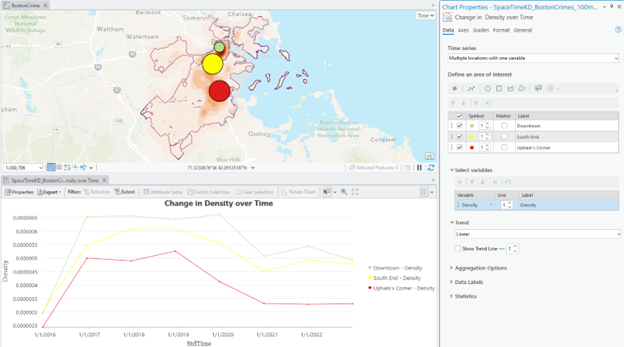
Understanding the distribution and clustering of events across space and time offers new, elevated insights and makes the decision-making process much simpler. While different tools offer unique advantages over one another, it is important to identify the appropriate tool based on the intended purpose of the analysis. It is also important to examine parameter values used in creating the output density surface and interpreting the output density surface. For example, while this example used the crime incidents and 311 call datasets for density calculations, it does not offer insights related to different classes of incidents. The output density surface is also impacted if the original data has any inherent bias or inaccuracies.
Use the table below to compare the Point Density, Kernel Density, and Space Time Kernel Density tools and how they differ from each other.
| Feature | Point Density | Kernel Density | Space Time Kernel Density |
| Definition | Calculates the number of points within a specified area. | Smooths out data using a kernel function to create a continuous surface | Incorporates both spatial and temporal dimensions to analyze point patterns over time and elevation |
| Calculation method | Simple count of points within a defined area. | Uses a kernel function to spread points over a surface where density values are higher closer to the center | Considers both spatial and temporal dimensions and uses a kernel function for each dimension to calculate the density over the surface |
| Output type | 2D raster showing point distribution. | 2D continuous raster surface showing density values | Multidimensional raster with optional voxel layer |
| Time | Does not consider temporal aspects. | Does not consider temporal aspects | Considers temporal distribution and changes in patterns |
| Elevation | Not considered | Not considered | Considers elevation in calculating density and creating multidimensional output raster with varying elevations |
| Multidimensional Output | Not supported | Not supported | Always creates a multidimensional raster |
| NetCDF support | Not supported | Not supported | Supports creation of NetCDF output raster with (.nc) filename extension |
| Voxel Layer support | Not supported | Not supported | Creates an optional voxel layer if the output raster is declared as NetCDF |
| Barrier | Not supported | Available to use polyline or polygon. Sketch function available to draw barriers. | Not supported |
| Distance decay effect | Not considered. Uniform weights for all input points within the neighborhood irrespective of distance from source. | Considered | Considered in all dimensions |
| Search window (Bandwidth) | Not supported | Supported only for 2D operations | Supported for all dimensions including time and elevation |
| Kernel Type | Not supported, uses four neighborhood types | Uses Quartic kernel type by default | Uses Quartic kernel type by default |
Learn more
This is the first in a series of five blog articles introducing you to a new approach to understanding density analysis. The next blog article will describe how to use the Space Time Kernel Density tool to create a NetCDF output raster and voxel layer for 3D exploration and visualization. It will include examples using climatic and oceanographic data and explore how to use the extended capabilities of the tool and, by extension, ArcGIS Pro to better understand the distribution of density across elevation (z-dimension) and time (t-dimension).
In future updates, the Density toolset will continue to add new capabilities to multiple ArcGIS products, including ArcGIS Pro, ArcGIS Online, ArcGIS Image Server, ArcGIS Enterprise, and ArcGIS Enterprise on Kubernetes. If you are interested in learning more about density tools, see the following conceptual documentation and be on the lookout for future blog articles focusing on Density tools:
- Understand density analysis
- How Kernel Density works
- How Space Time Kernel Density works
- Difference between point, line, and kernel density
Data source
The Crime Incident Reports and 311 Service Requests data used here was collected from Analyze Boston.
References
- 311 Service Requests – Analyze Boston. (2024). Boston.gov. https://data.boston.gov/dataset/311-service-requests
- Crime Incident Reports (August 2015 – To Date) (Source: New System) – Analyze Boston. (2024). Boston.gov. https://data.boston.gov/dataset/crime-incident-reports-august-2015-to-date-source-new-system

Article Discussion: