This blog article was originally published on August 20, 2024, and has been updated.
Jointly managed by NASA and the USGS, Landsat is the longest running spaceborne earth imaging and observation program in history. The Landsat program began in 1972, with the launch of Landsat 1. Beginning with Landsat 4, the program began providing mission to mission data continuity.
The Landsat Level-2 multispectral imagery is available in ArcGIS Living Atlas of the World as a time enabled image service, accessible across the ArcGIS system. For more about the service and the data, see Landsat Level-2.
This learning tutorial steps you through using Landsat Explorer to investigate and unlock the wealth of information that Landsat imagery provides.
Quick Links
Use the links below to jump to sections of interest.
Introduction
Explore
Compare
Analyze
- Analyze – Index mask
- Analyze – Temporal profile
- Analyze – Spectral profile
- Analyze – Change detection
Introduction
About Landsat missions
Since 1972, Landsat satellites have continuously acquired space-based images of the Earth’s land surface as part of the U.S. Geological Survey (USGS) National Land Imaging (NLI) Program.
This imagery provides uninterrupted data to help land managers and policymakers make informed decisions about our natural resources and the environment. Landsat Missions have been imaging the earth since 1972. For more information, see Landsat Satellite Missions.

Landsat Explorer essentials
Landsat Explorer is an ArcGIS Living Atlas app that enables you to investigate and unlock the wealth of information that Landsat provides.

The app offers key capabilities, including the following:
- Visual exploration of a dynamic global mosaic of the best available Landsat scenes.
- On-the-fly multispectral band combinations and indices for visualization and analysis.
- Interactive Find a Scene by location, sensor, time, and cloud cover.
- Visual change by time, and comparison of different renderings, with Swipe and Animation modes.
- Analysis such as threshold masking and temporal profiles for vegetation, water, land surface temperature, and more.
Note that Landsat 7 suffered a significant technical setback in 2003, resulting in data gaps in all subsequent images that mission collected. It continued to collect images until 2022 and these images are included in the archive. If you wish to filter for specific missions to include in the list of available scenes, you can do so using the Mission filter found at the top of the Scene Selection calendar.
Open the app
Landsat Explorer can be opened from the ArcGIS Living Atlas Apps page, found in the Apps tab at the Living Atlas Home. The app can also be opened directly from the Landsat Explorer item overview. The overview provides additional information about the app and the Landsat program.
Essential tools
The following tools are always available and can be used to navigate, share, make screen captures, and more.
In the upper left you’ll find tools to learn more about the app, zoom, and also the following:
a – Zoom to Landsat imagery native pixel resolution.
b – Zoom to the full extent of the imagery.
c – Capture the current map view as an image.
d – Copy a link to the app in its current state. This is a useful way to save all settings and share your work.

In the upper right you can toggle the visibility of map labels, terrain, and the basemap. Below that, a search tool enables you to find an address or a place.

Explore
Dynamic view mode
The app opens in dynamic view mode by default. In this mode, the most recent and most cloud free scenes from the Landsat archive are prioritized and dynamically fused into a single mosaicked image layer. As you pan and zoom, the map continues to dynamically fetch and render the best available scenes.
Landsat Explorer opens to one of several interesting places, each using a different renderer that most effectively highlights specific characteristics of the imagery. You can select and learn more about these locations by following the steps below.
Step 1 – Open Landsat Explorer. The app opens to an interesting place in dynamic view mode using a renderer, as indicated by the selected (highlighted) cards. Below, the app has opened to Kalahari Dunes using the Geology renderer.

Step 2 – Hover over any card in Interesting Places to learn more about the place. Click the card to zoom to the place.

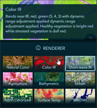
Landsat sensors collect imagery at distinct ranges along the electromagnetic spectrum. These bands of imagery can be combined to create renderings of the earth that highlight certain characteristics of the imagery and reveal additional information.
Step 3 – Hover over any renderer to learn more about it. Click to apply the renderer to the imagery.
Step 4 – Click anywhere on the map to get more information about the Landsat imagery, such as mission, date, temperature, and more.

In the next section, you will use tools and settings described above to learn more about a specific place.
Step 5 – From Interesting Places, choose Quelccaya. Hover over the card to learn more about the area.
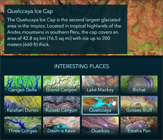
Note that when Quelccaya is displayed, the Short-wave IR renderer is applied automatically, highlighting the glacier in blue tones.
Step 6 – Click anywhere on the glacier and view the information. Next, click on a different area of the map, away from the glacier. Compare the information about the areas, especially temperature.

Step 7 – Change the renderer to Surface Temp and view the colorized surface temperature scale. This renderer uses the temperature values from the imagery and displays the map with red tones being warmer and white to blue tones being colder.
Step 8 – Change the renderer to Modified Normalized Difference Water Index (MNDWI) and view the water index scale. This renderer shows the driest areas in white to light tan and high water content areas in deep blue.

Step 9 – Explore further using other locations and renderers. Use the search tool to find other locations of interest.
Step 10 – Use the Copy link tool described in the About Landsat Explorer section to capture the current state of your map as you explore. Here are some examples:
Quelccaya ice cap using Surface Temp renderer
Quelccaya ice cap using MNDWI renderer
California Central Valley using Agriculture renderer
Cortina d’Ampezzo, Belluna, Italy using NDVI Colorized renderer
Find a scene
This mode allows for the selection of individual Landsat scenes by year, month, and day.
In the next exercise, you will find scenes that cover the 2022 eruption of Mauna Loa, the world’s largest active volcano located on the island of Hawaiʻi in the state of Hawaiʻi. The eruption began in the summit caldera of the volcano on November 27, 2022, and ended on December 13, 2022.
Step 1 – Click the button below to open Landsat Explorer to the area near the Mauna Loa summit caldera in dynamic view mode with the Natural Color renderer.

Step 2 – Click Find A Scene to switch to scene mode.

The Scene Selection calendar appears showing available Landsat scenes over the past 12 months. Filters at the top of the calendar enable you find scenes by mission or by cloud cover.
The scenes matching your criteria are included in the calendar and those meeting the specified cloud cover tolerance and mission are highlighted with a solid fill.

To learn more about a specific scene, hover over a square to view the scene information tip.

Next, you will find available scenes around the time of the eruption: November 27, 2022 to December 13, 2022
Step 3 – Click the date drop-down and select 2022 to find available scenes for that year.

Step 4 – View the available scenes. All available November scenes for that location were captured prior to the eruption, so find the next available scene in December. Hover over the square for more information, and click the square to add the scene to the map.

Once selected and added to the map, detailed scene information is displayed to the right of the calendar in the Scene Information panel.

Step 5 – Choose a different renderer to highlight the lava flow. Experiment with with Color IR, Short-wave IR, Urban, and others to find one that delivers the best visualization. Here are examples:
Step 6 – Click anywhere on the lava flow and view the information. Next, click on a different area of the map away from the flow. Compare the information about the areas, especially temperature.

The Find A Scene workflow is leveraged throughout the rest of the app, simplifying the discovery and selection of scenes.
Step 7 – Click the image below to compare with your map, or open Landsat Explorer with the exercise settings above.

Compare
Use swipe to compare scenes
In Swipe mode, you can select two scenes to swipe and visually compare differences between them. It is common to choose between scenes of different dates, but you can also swipe and compare different renderings of the same date, or mix and match the two. Swipe is a simple yet extremely powerful way to visually detect, explore, and analyze differences and similarities between two images.
In the next exercise, you will find and compare scenes of the May 2023 Long Lake Fire in Alberta, Canada, comparing before and after fire conditions.
Step 1 – Click the button below to open Landsat Explorer in dynamic mode to the area encompassing the fire.
Step 2 – Click Swipe to switch to scene swipe mode.

The stacked Left and Right boxes indicate the scenes selected for the left and right sides of the swipe.
Step 3 – Click Left and following the scene selection workflow described in the previous section, select the scene for August 19, 2022. This is the pre-fire Landsat scene.
Step 4 – Choose the Short-wave IR renderer for the scene.
Step 5 – Click Right and following the scene selection workflow used in Step 3, select the scene for September 15, 2023.
Step 6 – Choose the Short-wave IR renderer for the scene. Your swipe should be configures as shown below:

Step 7 – Use the swipe tool to compare the two scenes. The image on the left shows pre-fire conditions, while the image on the right is post-fire, where the burn scars are readily visible as a fuchsia color in this Short-wave Infrared spectral rendering.
Step 8 – Click the image below to compare with your map, or open Landsat Explorer with the exercise settings.

Animate multiple scenes
In Animate mode, you can select multiple scenes to create compelling time animations. When you have gathered your collection of images, click the play button to start the animation. During playback, you can choose your frame rate and optionally export your animation to an MP4 with the layout of your choosing.
In the next exercise, you will animate urban sprawl and construction in Dubai, United Arab Emirates, one of the fastest growing urban areas in the world.
Step 1 – Click the button below to open Landsat Explorer to the area near Dubai in dynamic imagery mode.
Step 2 – Click Animate to switch to animate mode, then click Add A Scene.

Step 3 – Using the Scene Selection calendar, add the following scenes:
- April 1, 1991. Natural Color
- May 17, 2002, Natural Color
- September 30, 2002, Natural Color
- May 28, 2003, Natural Color
- February 15, 2024, Natural Color
Step 4 – When finished, click the arrow at the bottom of the scene list to play the animation.

Step 5 – Use the play controls to (from left to right):
- Adjust the animation speed.
- Capture a link to the animation.
- Download the animation as an MP4 file.
- Pause/Play.
- Dismiss the play controls.

Step 6 – Click the image below to compare with your map, or open Landsat Explorer with the exercise settings.

Analyze
Analyze: Index Mask
In this mode you can use spectral indices, mathematical combinations of spectral pixel values from multiple spectral bands in an image, to highlight the relative abundance of things like water, moisture, and vegetation. As you move the index slider to adjust values, a mask is dynamically rendered on screen indicating the areas meeting the specified thresholds. Alternatively, the mask can be used to clip the image and only show the pixels covered by the mask.
In this next exercise, you will examine the water index and vegetation in the area around Boise, Idaho.
Step 1 – Click Analyze, then choose Index.

Step 2 – Choose an area of interest using the Search tool. Search for Boise, Idaho.

Step 3 – Using the Scene Selection calendar, choose a date. For this example, leave the date selector at Past 12 Months and choose March 16, 2024.

Step 4 – Render the imagery using the Agriculture renderer.
Step 5 – Zoom to the Landsat imagery native resolution. This is optional, but provides the best results.

Step 6 – Choose Water Index from the drop-down.
Step 7 – Adjust the slider to the desired values.
Step 8 – (Optional) Experiment using the Clip to mask and color options.

Step 9 – Use the Copy link tool to capture the current settings.
In the images below, the first shows the results from following the steps above. The areas with the highest water index are highlighted.
Click the image below to view a larger version, or open Landsat Explorer to the saved settings from the steps above.

The next image shows the areas of healthiest vegetation. Click the image to view a larger version, or open Landsat Explorer to the saved vegetation index settings.

The next image shows the areas of hottest surface temperature. Click the image to view a larger version, or open Landsat Explorer to the saved temperature index settings.

Analyze: Temporal Profile
Using the Temporal profile tool, you can detect categorical trends over time, including surface temperature as well as moisture, vegetation, and water.
In this next exercise, you will examine yearly and monthly temperature vs. moisture trends for an agricultural area near Sinop, Brazil.
Step 1 – Click Analyze, then choose Temporal profile.

Step 2 – Choose an area of interest using the Search tool.
Step 3 – Using the Scene Selection calendar, choose a date.
Step 4 – Choose a renderer for the imagery.
Step 5 – Zoom to the Landsat imagery native resolution.
Step 6 – Choose a Trend from the drop-down.
Step 7 – Choose Monthly or Yearly for the temporal profile.
When Yearly is selected, you can specify the target month you would like to be sampled year over year. This option is best for identifying long term patterns and trends. When Monthly is selected, you specify the target year and all 12-months within that year will be sampled. This option is useful for seeing seasonal patterns and fluctuations throughout the year.
Step 8 – Click anywhere on the map to generate the profile for that location.

Step 9 – Choose another trend to view the correlation between them. For example, this comparison shows yearly trends in surface temperature vs. moisture vs. vegetation.

This comparison shows monthly trend in surface temperature vs. moisture vs. vegetation.

The example below shows the yearly vegetation trend for a location near Matupo, Brazil. Click the image to view a larger version, or open Landsat Explorer to the saved yearly vegetation trend. Experiment using other trends and scenes.

Analyze: Spectral Profile
Multispectral imagery like Landsat measures the varying amounts of light that different materials reflect, known as spectral responses. By repeatedly sampling the spectral response of the same type of material on the Earth’s surface it is possible to build a spectral signature for that material.
Using the spectral profile tool, you can click anywhere on the map and a spectral profile for that point will be generated. Simultaneously, we will try to match that selected point with one of the pre-defined spectral signatures available in the dropdown list.
To explore spectral profiles, the steps are similar to other analysis tools: click Analyze and select Spectral profile, choose a scene from the Scene Selection calendar, choose a renderer, then click anywhere on the map.
Shown below is an example near Kearney, Nebraska that has been identified as healthy vegetation. Click the image to view a larger version, or open Landsat Explorer to the saved spectral profile. Experiment using other locations and profiles.

Analyze: Change Detection
Using Change detection, you can select two scenes and calculate the difference between them. You can create change masks based on vegetation, water, and moisture indices. Creating difference images allows you to do further analysis, such as estimating forest and vegetation loss in the event of a wildfire.
The next exercise uses the two Alberta, Canada, wildfire scenes used in the swipe section above. You will examine the difference in the vegetation index for each image and and create a difference mask
Step 1 – Click the button below to open Landsat Explorer in dynamic mode to the area encompassing the fire.
Step 2 – Click Analyze, then choose Change detection.

Scene A will be compared to Scene B when you click View Change.
Step 3 – Click Scene A and using the Scene Selection calendar choose August 19, 2022. Render the scene using the Short-wave IR renderer.
Step 4 – Click Scene B and using the Scene Selection calendar choose September 15, 2023. Render the scene using the Short-wave IR renderer.
Step 5 – Click View Change Scene A – Scene B.

Step 5 – Choose Vegetation Index from the Change drop-down. Adjust the slider to mask areas where vegetation has decreased.

Click the image below to view a larger version, or open Landsat Explorer to the saved change detection. Experiment using other locations and settings.

More information
For more information, see the following:


Commenting is not enabled for this article.