Map Predominant Disadvantage with Justice40 Data Using ArcGIS API for Python

The Justice40 Initiative is a federal effort to ensure that 40 percent of the benefits from federal investments reach disadvantaged communities across the United States. It targets inequities in eight key areas: Climate Change, Clean Energy, Clean Transit, Affordable Housing, Workforce Development, Legacy Pollution, Health Burdens, and Clean Water Infrastructure. 

Esri has integrated the Justice40 Tracts from Council on Environmental Quality (CEQ) into ArcGIS Living Atlas of the World, enabling detailed mapping and analysis of these disadvantaged communities across the U.S. and its territories. By leveraging this data in ArcGIS, users can create maps that identify these communities and support deeper analysis and targeted interventions. 

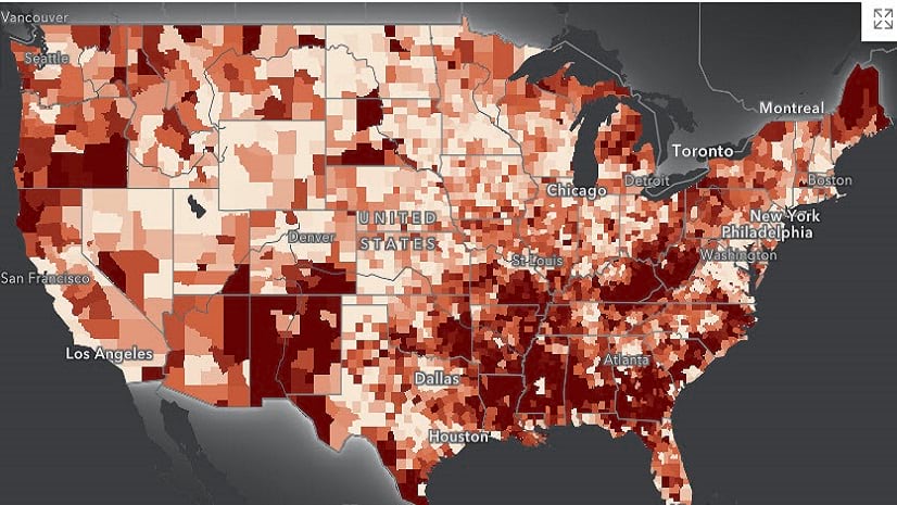
Because many policy decisions and resource allocations occur at the county level, aggregating data from census tracts to counties ensures that analysis is directly applicable to the administrative units responsible for implementing policies. In this article, we will use the ArcGIS API for Python and Justice40 data from Esri to map the predominant disadvantage categories at the county level across the U.S.  

Importance of Identifying Predominant Disadvantage Category

Identifying the predominant disadvantage category for each county involves determining which issue—such as climate change, clean energy, housing, or health—most affects the census tracts within that county. This is crucial because it highlights the primary challenge impacting the largest portion of the population, enabling more focused and effective policy interventions. 

Additionally, aggregating racial and ethnic demographic data to the county level is essential for recognizing and addressing disparities. By analyzing the share of each racial and ethnic group within a county, policymakers can ensure that their efforts are inclusive and equitable, targeting the needs of all community members, particularly those who have been historically marginalized. 

Overall, understanding the predominant disadvantage category in a county helps policymakers: 

• Prioritize resources: Allocate attention and funding to the most pressing issues within each county. 

• Develop targeted strategies: Tailor policies and programs to address the specific needs identified within the county. 

• Promote equity: Ensure that interventions are designed with a clear understanding of which communities and demographic groups are most affected. 

To create a map that visualizes the predominant disadvantage categories in U.S. counties using Justice40 data, we will follow these five steps: 

Step 1: Import Required Libraries and Access Justice40 Data 

First, we import the necessary libraries and connect to ArcGIS Online to access the Justice40 data. 

import pandas as pd
from arcgis.gis import GIS

# Connect to ArcGIS Online account
gis = GIS("https://www.arcgis.com", "username", "password")

# Retrieve the Justice40 data layer from ArcGIS Online
item_id = 'f95344889cab44bd84207052f44cb940'
justice = gis.content.get(item_id)
justice_layer = justice.layers[0]

# Display available layers
print("\n".join([f"{lyr.properties.id}: {lyr.properties.name}" for lyr in justice.layers]))

 Step 2: Query and Prepare Tract-Level Data 

Next, we query the Justice40 data layer to retrieve data fields including population, disadvantage categories, and racial demographics. We then prepare this data for aggregation to the county level by adding essential columns, such as the county FIPS code and calculated fields like the number of people affected in each demographic group. 

# Query the layer and convert to Spatially Enabled DataFrame 
lyr_df = justice_layer.query(out_fields=['GEOID10', 'SF', 'CF', 'TPF', 'N_WTR', 'N_WKFC', 'N_CLT', 'N_ENY', 'N_TRN', 'N_HSG', 'N_PLN', 'N_HLTH', 'CC', 'SN_C', 'DM_B', 'DM_AI', 'DM_A', 'DM_HI', 'DM_W', 'DM_H', 'DM_T'], out_sr=4326).sdf 

# First, ensure GEOID10 is a string
lyr_df1['GEOID10'] = lyr_df1['GEOID10'].astype(str)

# Extract the first 5 characters to get the state+county FIPS code
lyr_df1['FIPS'] = lyr_df1['GEOID10'].str.slice(start=0, stop=5)

# Create new columns for racial and demographic calculations 
lyr_df['African American'] = lyr_df['TPF'] * lyr_df['DM_B'] 
lyr_df['White'] = lyr_df['TPF'] * lyr_df['DM_W'] 
lyr_df['Asian'] = lyr_df['TPF'] * lyr_df['DM_A'] 
lyr_df['Hispanic'] = lyr_df['TPF'] * lyr_df['DM_H'] 
lyr_df['American Indian'] = lyr_df['TPF'] * lyr_df['DM_AI'] 
lyr_df['Native Hawaiian or Pacific'] = lyr_df['TPF'] * lyr_df['DM_HI'] 
lyr_df['Two or more races'] = lyr_df['TPF'] * lyr_df['DM_T'] 
lyr_df['Pop_in_Disadv_Tracts'] = lyr_df['TPF'] * lyr_df['SN_C'] 
lyr_df['FIPS'] = lyr_df['GEOID10'].str.slice(start=0, stop=5) 
lyr_df['Total_Tracts_Per_County'] = lyr_df.groupby('FIPS')['FIPS'].transform('size')

 Step 3: Aggregate Data to County Level 

In this step, we aggregate the tract-level data to the county level to identify the predominant disadvantage category for each county. This is crucial for understanding which issues are most prevalent in each county in the U.S., allowing for targeted interventions. We also calculate the percentage of different racial and ethnic groups within each county. This helps ensure that the analysis considers the diverse populations affected by the disadvantages.

# Aggregate data at the county level 
county_level_df = lyr_df.groupby(['FIPS', 'SF', 'CF']).agg({ 
    'TPF': 'sum', 
    'N_WTR': 'sum', 
    'N_WKFC': 'sum', 
    'N_CLT': 'sum', 
    'N_ENY': 'sum', 
    'N_TRN': 'sum', 
    'N_HSG': 'sum', 
    'N_PLN': 'sum', 
    'N_HLTH': 'sum', 
    'SN_C': 'sum', 
    'African American': 'sum', 
    'White': 'sum', 
    'Asian': 'sum', 
    'Hispanic': 'sum', 
    'American Indian': 'sum', 
    'Native Hawaiian or Pacific': 'sum', 
    'Two or more races': 'sum', 
    'Pop_in_Disadv_Tracts': 'sum', 
    'Total_Tracts_Per_County': 'first' 
}).reset_index()

# Calculate share of population in disadvantaged tracts and demographic percentages 
county_level_df['Share_of_Pop_in_Disadv_Tracts'] = county_level_df['Pop_in_Disadv_Tracts'] / county_level_df['TPF'] 
county_level_df['Share_of_African Americans'] = county_level_df['African American'] / county_level_df['TPF']
county_level_df['Share_of_Whites'] = county_level_df['White'] / county_level_df['TPF'] 
county_level_df['Share_of_Hispanics'] = county_level_df['Hispanic'] / county_level_df['TPF'] 
county_level_df['Share_of_Asians'] = county_level_df['Asian'] / county_level_df['TPF'] 
county_level_df['Share_of_American_Indians'] = county_level_df['American Indian'] / county_level_df['TPF']
county_level_df['Share_of_Native_Hawaiians'] = county_level_df['Native Hawaiian or Pacific'] /county_level_df['TPF'] 
county_level_df['Share_of_Two_or_more races'] = county_level_df['Two or more races'] / county_level_df['TPF']

Step 4: Identify the Predominant Disadvantage Category 

Here, we identify the predominant disadvantage category for each county by determining which category is most prevalent. The function,find_predominant_category_explicit , determines the predominant disadvantage category for each county. It checks whether the county has any disadvantaged tracts using the Has_Disadv_Tract flag. If there are no disadvantaged tracts, it returns “No Disadvantaged Tracts.” Otherwise, it iterates through each disadvantage category to find the one with the highest impact (i.e., the highest value). The function then returns the full name of the predominant category.

# Create a flag for counties with disadvantaged tracts 
county_level_df['Has_Disadv_Tract'] = county_level_df['SN_C'] > 0 

# Define disadvantage categories and their names 
disadvantage_categories = ['N_WTR', 'N_WKFC', 'N_CLT', 'N_ENY', 'N_TRN', 'N_HSG', 'N_PLN', 'N_HLTH'] 

category_names = { 
    'N_WTR': 'Water and Wastewater Disadvantaged', 
    'N_WKFC': 'Workforce Development Disadvantaged', 
    'N_CLT': 'Climate Change Disadvantaged', 
    'N_ENY': 'Energy Disadvantaged', 
    'N_TRN': 'Transportation Disadvantaged', 
    'N_HSG': 'Housing Disadvantaged', 
    'N_PLN': 'Legacy Pollution Disadvantaged', 
    'N_HLTH': 'Health Disadvantaged'} 

# Function to find predominant disadvantage category 
def find_predominant_category_explicit(row): 
    if not row['Has_Disadv_Tract']: 
        return "No Disadvantaged Tracts" 
    max_value = -1 
    max_category = None 
    for category in disadvantage_categories: 
        category_value = row[category] if pd.notnull(row[category]) else 0 
        if category_value > max_value: 
            max_value = category_value 
            max_category = category 
    return category_names[max_category] if max_category else "No Disadvantaged Tracts" 

# Apply the function to determine predominant category 
county_level_df['Predominant_Disadvantage'] = county_level_df.apply(find_predominant_category_explicit, axis=1)

Step 5: Merge with County Boundaries and Publish as a Feature Layer 

Finally, we merge the aggregated county-level data with geographic boundary data for each county. After merging, the dataset is published as a feature layer in ArcGIS, allowing for interactive analysis and visualization. This step ensures that the insights gained from the data are easily accessible and actionable, providing a valuable tool for policymakers and stakeholders.

# Access county boundaries and merge with data 
county = gis.content.get('1f60b7a2c9f748909834367ed33197fd').layers[1] 
county_df = county.query(out_fields=['GEOID10'], out_sr=4326).sdf 
county_df.rename(columns={'GEOID10': 'FIPS'}, inplace=True)  

# Merge the county-level data with the county boundaries 
merged_df = pd.merge(county_level_df, county_df, on='FIPS', how='right') 
merged_df.spatial.set_geometry('SHAPE', inplace=True) 

# Rename columns to ensure valid field names 
merged_df.columns = [col.replace(' ', '_').replace('-', '_') for col in merged_df.columns] 

# Publish the merged data as a feature layer 
item_properties = { 
    "title": "County Predominant Disadvantage Category", 
    "description": "This layer highlights the primary category of disadvantage for each county in the United States, based on the Justice40 Initiative.", 
    "tags": ["Justice40", "disadvantage", "data science", "county level analysis"] 
} 

# Publish as a feature layer to ArcGIS Online 
feature_layer_item = merged_df.spatial.to_featurelayer( 
    title=item_properties['title'],  
    gis=gis,  
    tags=item_properties['tags'],  
    description=item_properties['description'] 
)  
print(f"Feature Layer created: {feature_layer_item.url}")

You can access the final map through this link. 

Conclusion 

In this workflow, we used the ArcGIS API for Python to efficiently access, analyze, and visualize Justice40 data. By aggregating data from census tracts to counties, we identified key disadvantage categories and highlighted affected demographic groups at the county level. This aggregation is particularly important because it aligns with the administrative units where many policy decisions and resource allocations are made. This streamlined process not only simplifies complex data analysis but also supports data-driven policy decisions, ensuring resources are allocated where they are most needed. The ArcGIS API for Python is a powerful tool for quick, seamless workflows that enhance the effectiveness and precision of policy-making.