In ArcGIS Pro 3.4, we released a new tool Create Spatial Component Explanatory Variables which can create variables that effectively account for the confounding nature of spatial data in machine learning.
Creating Spatial Components
In many cases, there are unmeasured spatial processes that can wreak havoc in our predictive models!
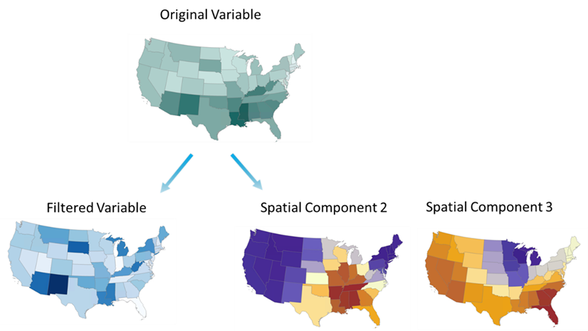
The Create Spatial Component Explanatory Variables tool can help create variables that account for the unmeasured spatial patterns that may be present in your dataset. It does so by creating spatial components based solely on the arrangement of the geometry in your dataset. The tool selects the subset of spatial components that best predict a numeric variable.
To illustrate, we will use the famous Ames housing dataset (De Cock, 2011) to illustrate how this tool works. We want to predict the price of houses being sold in Ames, Iowa.
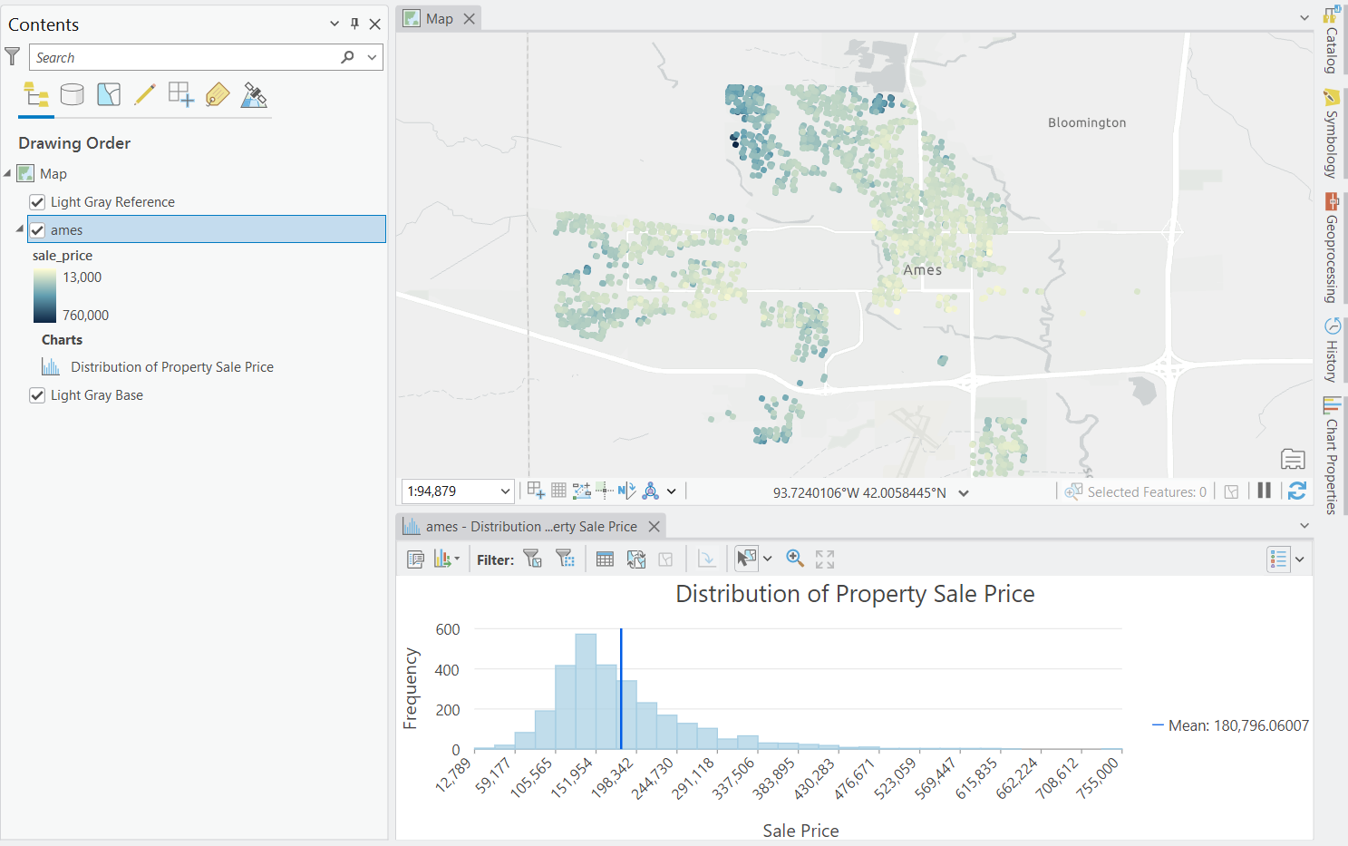
The average sale price in the dataset is just around $180,000. However, there is a very long tail where the 95th percentile of house sales are priced at $335,000. Looking at the variable we can see a fair amount of spatial clustering in housing price which traditional machine learning models may not be able to handle very well.
Predicting housing prices with Boosted Regression
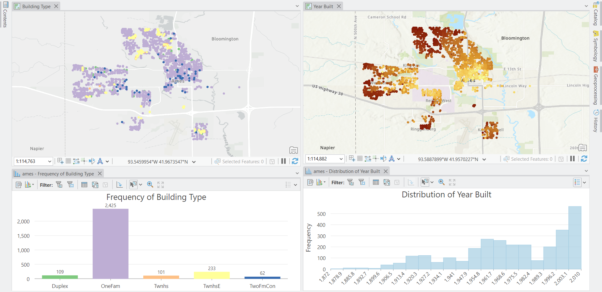
We will create a baseline model that uses the Forest-based and Boosted Classification and Regression tool from the Spatial Statistics toolbox. This baseline model will predict the sale price based on the type of building that is sold as well as the year that the property was built.
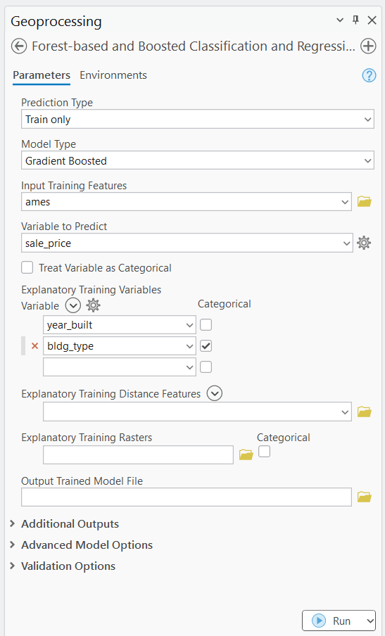
Open the Forest-based and Boosted Classification and Regression tool. We will pass in the Ames dataset and choose the sale_price as our dependent variable and the year_built and bldg_type as our independent variables. Additionally, we will use Gradient Boosted as our Model type.
After the model has trained, we can review the geoprocessing messages to assess the baseline model’s overall performance.
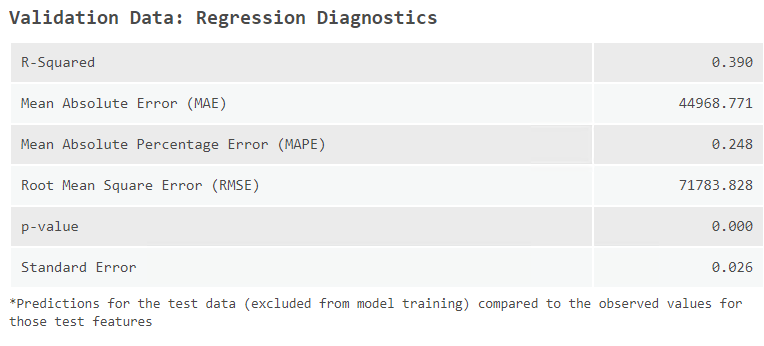
The validation diagnostics shows how our baseline model performs on out of sample data. The results are not the most impressive with an R-squared of only 0.39 and a mean absolute error of almost $45,000 dollars.

What is also quite interesting is that the bldg_type variable has a large weight importance meaning it is used a lot to help make branching decisions in our model.
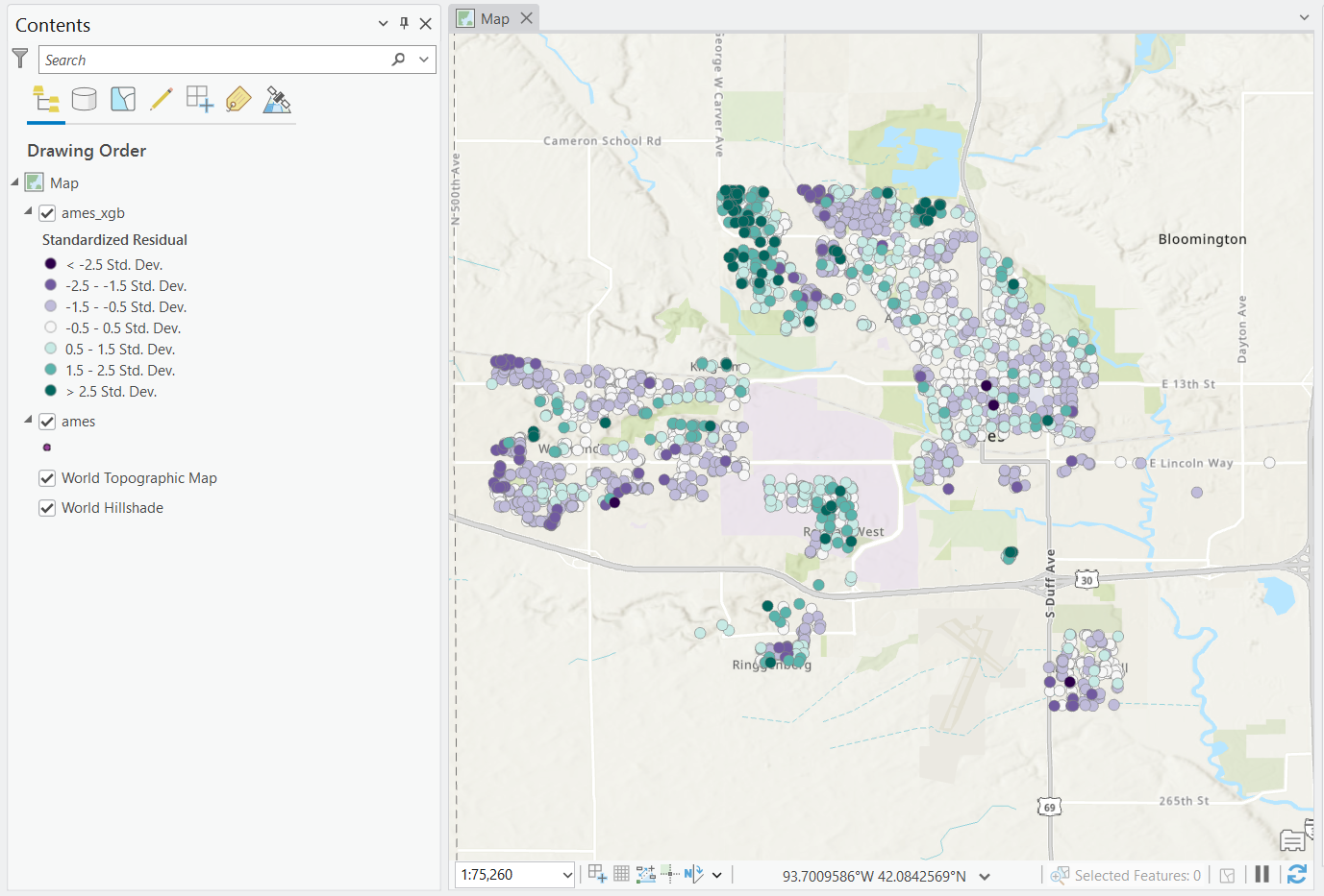
We can also see that there are quite extreme pockets of residuals throughout the corners of the map. Perhaps spatial heterogeneity is at play here and we need to better account for it.
Creating spatial components
To improve the quality of this model, we will create spatial components that are most predictive of sale_price. To do so, open the Create Spatial Component Explanatory Variables tool and use ames as the Input Features and the sale_price as the Input Fields.
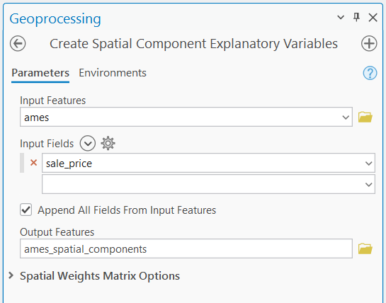
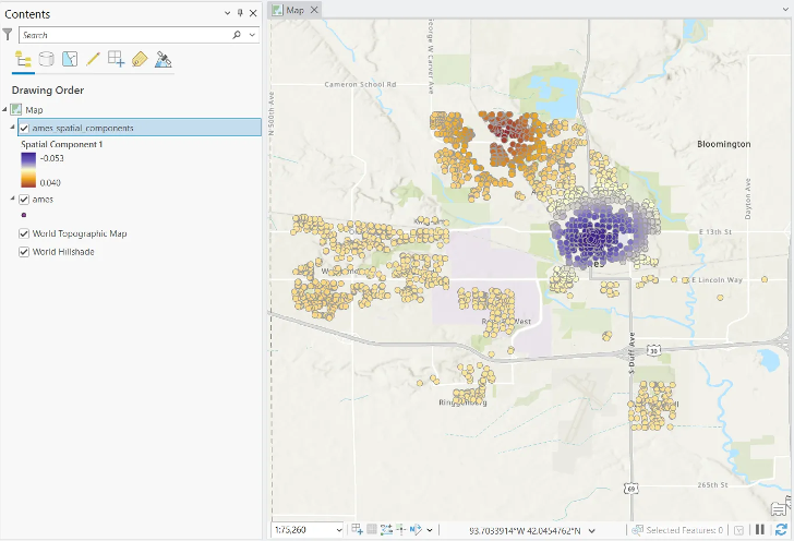
This tool will run through 28 possible spatial weights matrix configurations to identify the spatial weights matrix and combination of spatial components that are most predictive (using linear regression) of the sale_price variable. The output shows the first spatial component that was selected.
Incorporating space into our boosted tree-based model
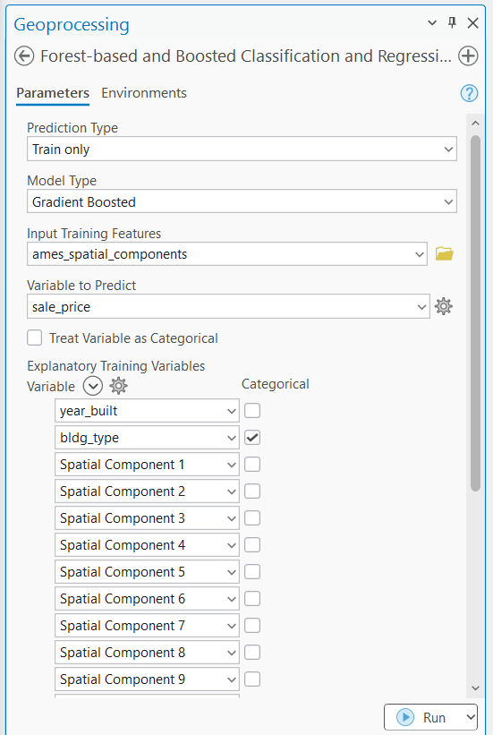
We can use these newly created components in our regression tree model to try and improve the performance. In the Explanatory Training Variables, include the first 10 components in addition to the original explanatory variables and run the tool again to train a new model.
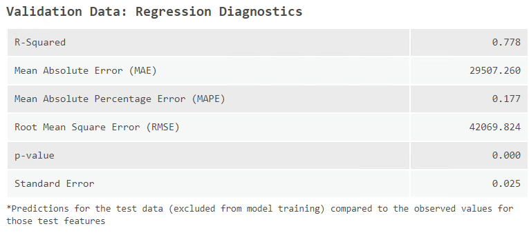
We can now review the performance of the new model which incorporates these spatial components. The validation R-squared has shot up by almost 0.4, almost doubling the variance explained by the regression model. This is a massive increase in model performance. Additionally, the mean absolute error (MAE) has been decreased from $45,000 to just under $30,000. That means that on average, the model’s predictions are almost $15,000 closer to the true value—that’s no small amount to laugh at
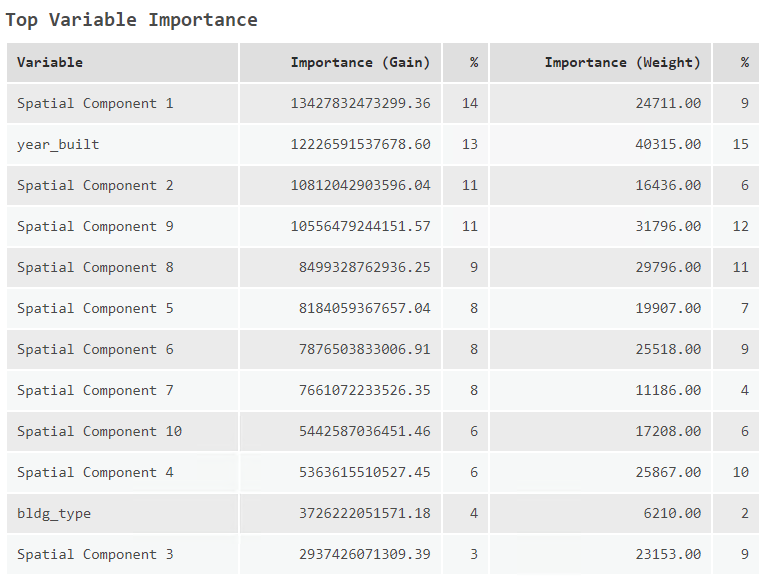
When looking at the importance of each of these variables, we can see that the year_built variable is still very important in calculating the the sale_price of a house. Now, though, the building type variable is arguably the least useful variable in the model!
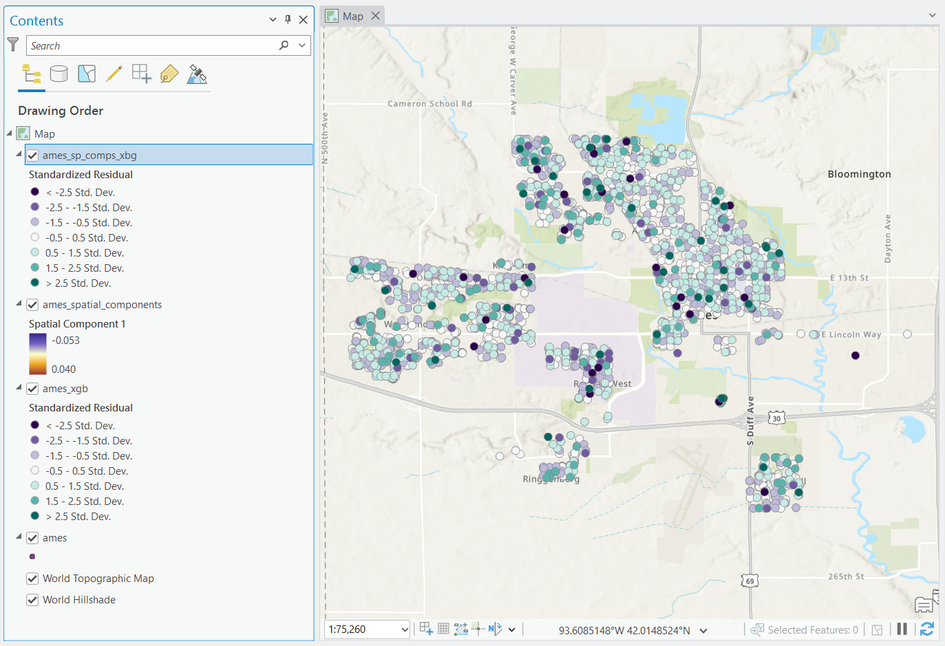
Lastly, when reviewing the model’s residuals, the residuals no longer appear to be spatially clustered. Rather, instead, they appear to be quite randomly distributed around the city itself.
Careful Considerations
By including spatial components into our model, we were able to greatly improve its predictive power. However, that doesn’t mean that they should be preferred. In fact, these spatial components are likely indicative of omitted variable bias (OVB).
When spatial components are useful in model predictions it is likely that there is some other real world phenomenon that the model is not taking into account. You can use these components to supplement your well measured variables, or even help you identify additional measures that you may need.
Citations
Tobler, W. R. 1970. “A Computer Movie Simulating Urban Growth in the Detroit Region.” Economic Geography 46: 234–40. https://doi.org/10.2307/143141.
Pebesma, E.; Bivand, R. (2023). Spatial Data Science: With Applications in R (1st ed.). 314 pages. Chapman and Hall/CRC, Boca Raton. https://doi.org/10.1201/9780429459016
De Cock, D. (2011) Ames, Iowa: Alternative to the Boston Housing Data as an End of Semester Regression Project. Journal of Statistics Education, 19, Published Online. https://doi.org/10.1080/10691898.2011.11889627
Article Discussion: