ArcUser Online

|
:
|
Crime analysts are making greater use of GIS to analyze and display geographic concentrations or hot spots of crime events. One of the techniques for performing this analysis is kernel estimation or kernel smoothing, a spatial statistical method that generates a map of density values from the point event data. A critical issue in the smoothing process is the selection of a bandwidth size or the radius of the circular window in which smoothing is performed. Most GIS and spatial statistical programs that perform kernel smoothing calculate the bandwidth based on the geographic extent of the point pattern. These estimates for bandwidth do not reflect the geographic distributions of the points within the study area, only their geographic extent. This can result in misleading density values and maps that are either too smooth or too spiky in appearance. This article describes a new approach for bandwidth estimation based on k-nearest neighbor distances between points. This method offers an improvement over existing methods because it is based on the spatial relationships among the points and thus reflects the degree of clustering and dispersion in the crime point pattern. This method of mapping crime density at different scales is illustrated using data from Brooklyn, New York.
Data Sources
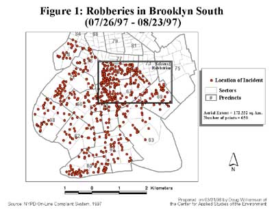
The data used in the analyses is from the New York City Police Department (NYPD) On-Line Complaint System. Each record corresponds to a location described by an address where a crime occurred. For the purpose of these analyses, only major felony incidents, as defined by the Federal Bureau of Investigation's Uniform Complaint Report, were used. The study, which was funded by a grant for the National Institute of Justice, focused on robbery and burglary data since these types of crimes are of major interest to the command structure of the NYPD. The incidents occurred during a 29-day period from July 26, 1997, to August 23, 1997. The study area is limited to the southern portion of Brooklyn, a borough in New York City. During the study period, this area recorded 650 robberies, as shown, and 873 burglaries. Kernel SmoothingThe goal of kernel smoothing is to estimate how the density of events varies across a study area based on a point pattern. "Kernel estimation was originally developed to obtain a smooth estimate of a univariate or multivariate probability density from an observed sample of observations..." (Bailey and Gatrell, 1995). In the spatial case, kernel smoothing creates a smooth map of density values in which the density at each location reflects the concentration of points in the surrounding area. In kernel estimation, a three-dimensional floating function visits every cell on a fine grid that has been overlaid on the study area. Distances are measured from the center of the grid cell to each observation that falls within a predefined region of i nfluence known as a bandwidth. Each observation contributes to the density value of that grid cell based on its distance from the center. Nearby observations are given more weight in the density calculation than those farther away. Kernel estimation has two advantages for displaying crime patterns. It clearly shows complex spatial point patterns in a smooth image that can also be used to create other data sets, and it can be used for quantitative comparisons over time. First, this method helps make sense of complex point patterns. The result, a smooth raster image of densities, can be used in conjunction with the point map. This means no information is lost in the analysis. From this raster image, users can quickly identify hot spots either by eyeballing (visually inspecting) them, which is subjective and very judgmental, or by defining hot spots based on statistical significance. The product of the kernel estimation method is a simple, aesthetically pleasing raster image from which users can derive other data sets, specifically contours of density. These contour loops can be displayed independently or they can be used to define the boundaries of hot spot areas that can then be analyzed separately. Hot spots are often irregular in shape. Unless the crime distribution is uniform the resulting contours will not be the circles or ellipses required in other crime clustering methods. Under kernel smoothing, the hot spots encompass a uniquely defined area and are not limited to any jurisdiction, or any man-made boundary for that matter. The hot spots may cover several separate entities such as police precincts or sectors or cut across political boundaries. Kernel estimation can also be used to analyze change over time. Raster images of crime density can be used as input into correlation analysis or time series analysis. The correlation analysis can be performed either by comparing two consecutive time periods (i.e., one month to the next) or by comparing one time period to a similar one (i.e., June of the current year to June of the previous year). Either way, the user would expect to see high values in an area from one period corresponding to high values in the same area for the other period. Time series/change analysis can use multiple density images to monitor change over time. One weakness in using the kernel estimator is the arbitrary nature of selecting a radius for the region of influence or bandwidth. There is no hard and fast rule for determining this distance, although some rules of thumb have been put forth. Ideally, this distance should represent the actual distances between points in the distribution. Estimating Bandwidth Selecting an appropriate bandwidth is a critical step in kernel estimation. The bandwidth determines the amount of smoothing of the point pattern. The bandwidth defines the radius of the circle centered on each grid cell, containing the points that contribute to the density calculation. In general, a large bandwidth will result in a large amount of smoothing and low density values, producing a map that is generalized in appearance. In contrast, a small bandwidth will result in less smoothing, producing a map that depicts local variations in point densities. Using a very small bandwidth, the map approximates the original point pattern and is spiky in appearance. Several rules of thumb have been suggested for estimating bandwidth. ArcView GIS, the only GIS software to kernel estimation, uses a measure based on the areal extent of the point pattern as the default bandwidth. Specifically, the bandwidth is determined as the minimum dimension (x or y) of the extent of the point theme divided by 30, or min. (x,y)/30. Bailey and Gatrell suggest a bandwidth defined by 0.68 times the number of points raised to the -0.2 power scaled to the areal extent of the study area, or 0.68(n)-0.2 . This can be adjusted depending on the size of the study area by multiplying by the square root of the study area size. The problem with both of these procedures for estimating bandwidth is that neither takes into account the spatial distribution of the points. Bailey and Gatrell's estimate is based on point density, but this is limited at best. Large sample sizes will result in small bandwidths, while small sample sizes will result in large bandwidths. No consideration is given to the relative spacing of the points. The arbitrary nature of the coefficient and power is also problematic. A very large number of combinations would yield similar results. The ArcView GIS default is also arbitrary. Dividing by the number 30 appears to have no statistical basis. A more practical approach to selecting a bandwidth would take into consideration the relative distribution of points across the study area. One way to achieve this is to base the bandwidth on average distances among points.
This study estimated bandwidth as the average kth nearest neighbor distance among points. The k-nearest neighbor approach is superior to other methods for selecting a bandwidth because it is based on the interpoint distances of the point pattern. Thus, the bandwidth will reflect the spacing of points rather than the size of the study area or the number of points. The proposed approach also adds flexibility to the kernel estimation procedure by allowing the user to vary k, depending on how much smoothing is desired. Instead of experimenting with different bandwidths in an ad hoc way, the user controls the degree of smoothing through the choice of k. The calculation of the k-nearest neighbor distance was performed using Avenue, the programming language for ArcView GIS. The procedure is relatively straightforward. First, the distances between each point and every other point are calculated. Then, using a nested loop structure, the distances for each point are sorted, and the average distance of the k-nearest neighbors is calculated. Then, in another loop, the average of those distances is calculated. The result is the recommended bandwidth based on k. Results Using This Method
The k-nearest neighbor approach was implemented on the burglary and robbery data at two geographical scales.
First, the two crimes were analyzed for Brooklyn South for the given time period.
The data presented above clearly indicates the differences between the ArcView GIS default bandwidth, Bailey and Gatrell's rule of thumb, and the values computed based on the k-nearest neighbor technique. The ArcView GIS default is useful when the study area is large as shown in Figure 3, but when a small study area is analyzed the default bandwidth becomes too small as in Figure 4. The density map when using a bandwidth that is too small will be spiky in appearance and have extremely high and low density values. 
Other problems occur if the study area is not square or close to square. If the study area is rectangular, with one side much longer than the other, the ArcView GIS default will use the smaller dimension in its bandwidth estimation. The result, again, will be a small bandwidth. An example of these types of problems can be illustrated by using the study area of Manhattan, in New York City, for which the Y dimension is approximately six times larger than the X dimension. Bailey and Gatrell's rule of thumb produces very large bandwidths, much larger than the default and nearest neighbor values. The end result is a highly smoothed map that does not show local variations in crime, but offers a generalized regional view. By comparison, bandwidths estimated by the nearest neighbor method are relatively stable with changes in scale as seen in Figures 5 and 6. Bandwidths for the subset data sets are roughly equal to those for the Brooklyn South data sets, for equivalent values of k. Thus, rather than being determined by the scale of the map, the bandwidth is based on the user-defined value of k.
Conclusions Kernel estimation has proved to be a useful tool in simplifying complex spatial point patterns. By creating a smooth of density values in which the density at each location reflects the concentration of points in the surrounding area, analysts are able to see how crime densities vary across a study area. However, the arbitrary nature of the process of selecting a bandwidth may result in misleading or inaccurate maps. The procedure proposed here, the k-nearest neighbor technique, bases the bandwidth on the spatial distribution of the point pattern, which maintains flexibility while empirically objectivity to the analysis. For more information, contact Doug Williamson by E-mail at dougwill@everest.hunter.cuny. Selected Bibliography Bailey, Trevor C. and Anthony C. Gatrell. Interactive Spatial Data Analysis. Reading, Massachusetts: Addison-Wesley Publishers, 1995.About the Authors Doug Williamson, a doctoral candidate at the City University of New York (CUNY), Graduate School and University Center, is a research associate for the Center for Applied Studies of the Environment of CUNY. His current research interests are the use of GIS in law enforcement, spatial statistics, and visualization. Sara McLafferty is associate professor of geography at Hunter College of the City University of New York. Her research interests include the use of GIS and spatial analysis methods in analyzing health and social issues. Victor Goldsmith is the acting dean of research, Hunter College of the City University of New York. John Mollenkop is the director for the Center for Urban Research of the City University of New York, Graduate School and University Center. Phil McGuire is the assistant commissioner for the Office of Management and Policy Planning of the New York City Police Department. |
 If dij is the distance from point i to its jth neighbor, then the average kth nearest neighbor distance is the formula
shown here. For example, if k is 10, the bandwidth is estimated as the average distance from each point to its 10 nearest neighbors.
The value of k is chosen by the analyst to specify the desired degree of smoothing of the data. Small k values result in
a small bandwidth, producing a spiky map with little smoothing. Larger k values result in a larger bandwidth and smoother
density map.
If dij is the distance from point i to its jth neighbor, then the average kth nearest neighbor distance is the formula
shown here. For example, if k is 10, the bandwidth is estimated as the average distance from each point to its 10 nearest neighbors.
The value of k is chosen by the analyst to specify the desired degree of smoothing of the data. Small k values result in
a small bandwidth, producing a spiky map with little smoothing. Larger k values result in a larger bandwidth and smoother
density map.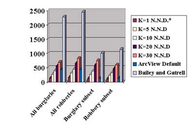 Second, by selecting out smaller geographic areas within the two larger data sets, subsets of these two data sets were created. The script was then
run on each of these data sets with varying k values. These results are summarized in this chart.
Second, by selecting out smaller geographic areas within the two larger data sets, subsets of these two data sets were created. The script was then
run on each of these data sets with varying k values. These results are summarized in this chart. The effect of using different k values is also important. Logically, it would follow that a higher k will yield a larger bandwidth
and a smaller k value will yield a smaller bandwidth. As k increases, the process searches larger areas for more nearest
neighbors, adding larger distances to the calculation. This is useful in providing a logical basis for how much smoothing is
desired. To use more points in smoothing use a larger k or, inversely, a smaller k for fewer points. The k value also can be
adjusted depending on the sample size (N). If N is small, a small k should be used; if N is large, a larger k should be tried.
The effect of using different k values is also important. Logically, it would follow that a higher k will yield a larger bandwidth
and a smaller k value will yield a smaller bandwidth. As k increases, the process searches larger areas for more nearest
neighbors, adding larger distances to the calculation. This is useful in providing a logical basis for how much smoothing is
desired. To use more points in smoothing use a larger k or, inversely, a smaller k for fewer points. The k value also can be
adjusted depending on the sample size (N). If N is small, a small k should be used; if N is large, a larger k should be tried.