Three ways to prepare your data for Voxel Layer

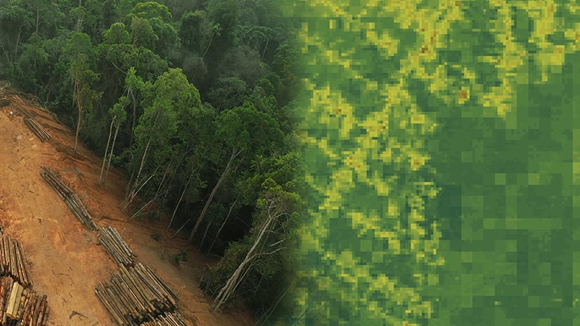
ArcGIS Pro 2.6 comes with a new Voxel functionality, allowing you to visualize 3D data grids with billions of voxel cubes while leveraging data filtering, symbology control customized for 3D data visualization, time animations and other interactive exploration features. From visualizing climate change modalities, marine ecosystems, geological phenomena to time-series of the digital divide, environmental and social justice metrics – this format of visualization can help convey critical information, provided the data is right.

Voxel Layer takes a specific type of NetCDF data as its input. The NetCDF format offers a lot of flexibility in terms of data storage. However, this flexibility also makes it the proverbial ‘wild wild west’ of data formats. The data needs to be compliant to the Voxel Layer data requirements to visualize it correctly as a voxel volume.

This blog demonstrates the use of Python to edit NetCDF files and make them compatible for voxel visualization. Most of these functionalities are also available in the raster object in ArcGIS Pro. There are additional tools for multidimensional data management and analysis available in ArcGIS Pro.

We will be using the Jupyter Notebook environment in ArcGIS Pro for the three types of data operations described in this blog. Open ArcGIS Pro, and open a new local scene. In the analysis tab, in the Geoprocessing group, select the Python option. A new Python notebook will open.

We are now ready to look at the three scenarios.

Combining a time series of netCDF files into a single netCDF

NetCDF data often come in separate files that span over different time stamps or height stamps, and often you might want to visualize this data as a Voxel layer with all individual time or height information combined into the same file. As an example, this precipitation data downloaded from the NOAA Physical Science Laboratory Server has netCDF files for different years, available to download separately.

So how may we go from disjointed netCDF files to a single netCDF file?

Create a folder with all the data that needs to be combined. Download the data from the PSL website listed above into this folder. I had a folder called ‘precip’ with the hourly precipitation data mentioned above. As in the screenshot, the data was named in this format — ‘precip.hour.yyyy.nc’, yyyy is the year of observation recording.

Now, for the code. First, import the xarray and netCDF4 libraries.

import netCDF4
import xarray

(Press Shift+Enter to execute the code in the Cell and open a new cell)

First, we need to confirm the name of the time dimension. We can do this by individually importing a single file, and checking its dimensions.

ds_precip = xr.open_dataset(r"\\qalab_server\vsdata\v27\Desktop\SceneLayers\data\NetCDF\X_Y_T\precip.hour.1981.nc")
ds_precip

We see in the results window that the time dimension is called ‘time’; Not all netCDF variables have such obviously relatable names, so it’s always good to check the name of the dimension.

We now need the script to open any netCDF file in my folder that begins with ‘precip.hour’, the * representing that whatever comes there is a don’t-care string. The way we want to combine the data is using the time coordinate dimension, which is the dimension that defines the relations of the data and order with respect to one another. These different precipitation data are input to the combine method, specifically by stating that we want to combine by the coordinate dimension – ‘time’ (combine = ‘by_coords’ and concat_dim = ‘time’ respectively). xarray provides more option to concatenate data with more complex needs like merging along two dimensions. For more, see here

ds_combined = xarray.open_mfdataset('precip.hour.*.nc',combine = 'by_coords', concat_dim="time")

We can now export this data into a combined netCDF,

ds_combined.to_netcdf('precip_combined.nc')

And now we can plot this data as a Voxel or a Spacetime Cube.

Reordering the dimensions in a netCDF data

CF compliance of NetCDF data does not impose restrictions on the order of the dimensions, so that data you need to visualize the Voxel layer with might not be ordered based on the requirements of the layer. In this situation, while loading netCDF data in the Add Voxel Layer dialogue, you may receive this warning

Warning : The order of the dimensions for variable ‘<variable name> ‘ is not supported. {X,Y,Z,T} or {T,Z,Y,X} order is expected (with z or t optional). Variable will be ignored.

This warning applies to latitude and longitude based dimensions as well, where the accepted order of dimensions is either {longitude, latitude, level, time} or {time, level, latitude, longitude}.

For instance if you take the relative humidity data here, which is based on the relative humidity data from NCEP/NCAR Reanalysis 1 data for relative humidity at multiple levels, daily averages for 2003.

When we try to add this data through the Add Multidimensional Voxel dialogue, no variables show up in the dialogue, and we get the same warning as above.

We need to transpose the data into the dimensions that the voxel layer accepts. You can use the same Jupyter Notebook opened above. Open the file with xarray.

import netCDF4
import xarray

ds_rhum = xarray.open_dataset(r"C:\Users\nee10059\Downloads\rhum.2003.nc")

We first check the coordinate dimension names by typing the dataset name.

ds_rhum

Now we will apply a mathematical array transpose operation to the data to be either ordered as {longitude, latitude, level, time} or {time, level, latitude, longitude}.

ds_ordered = ds_rhum.transpose("time", "level", "lat", "lon")

We can export this data into a reordered netcdf rhum_ordered.2003.nc

ds_ordered.to_netcdf(r"C:\Users\nee10059\Downloads\rhum_ordered.2003.nc")

We can now add this data to be visualized as a voxel.

Three ways to correct the direction of the height axis

NetCDF data may be misaligned along a particular dimension – x,y,z or t. In this case, we want to reverse (or un-reverse if you will) just the data along that axis while maintaining the structure along the others. The height dimension is the most susceptible of being stored in this reversed manner, but also commonly we might want to reverse the time dimension so that the spacetime cube voxel has the oldest timestamp as the topmost plane.

There are four cases in which the data may be aligned as shown in the figure. Consequently there are 24 permutations in which we might want to correct the direction of the alignment.
The data might be on the opposite side of the ground, and needs flipping (position (1) to position (4) above), or offsetting (position (1) to position (3)). Alternatively, the data might need to be reversed in direction while occupying the same geographical area  as before (position (position(1) to position (2)).

(Quick tip: If you do not want to manipulate the netCDF data itself and only the visualization, the voxel volume could be inverted through drawing manipulation. To do this, you can set a negative value in the ‘Vertical Exaggeration’ field in the Elevation group of the Appearance ribbon. Then use the offset field to position the volume above/below the earth surface.)

Let’s look at the Carbon monoxide reanalysis data from Copernicus Atmosphere Monitoring Service (CAMS) as Voxel volume, which was used in the figure above. The legend shows that the upper atmosphere has higher values of carbon monoxide, which reduce near the ground. An atmospheric expert would quickly understand that while the voxel volume is correctly placed geographically, the data is inverted.

We have to transform the data from position (1) to position (2) shown in Table 1.

We can use the same Jupyter notebook opened above in the ArcGIS Pro interface, import the necessary libraries and the data we will be working with.

import netCDF4
import xarray
ds_cams = xarray.open_dataset(r"C:\Users\nee10059\Downloads\Carbon_Monoxide_CAMS.nc")

We then find out the name of the height dimension, by typing the dataset name

ds_cams

The height dimension is called ‘level’. We can find out more attributes on the height dimension by clicking

ds_cams.level

The level dimension is ordered from 1 to 60, with a long name attribute of ‘model_level_number’.

From here, there are three steps to invert the netCDF data

1. 1. Reverse the data direction

      dnew = ds.reindex(level = list(reversed(ds.level)))

      This logic ‘reindexes’ or flips the data by reading it from a list created by reversing the ‘level’, and stores it in a new dataset dnew. dnew contains the reversed data but the level misaligned, i.e. level 1 (ground) now contains level 60’s information.

   2. Rename the ‘level’ numbering to align with the original netcdf array

      dnew = dnew.assign_coords(level = ds.level)

   3. Supply attribute information.
      The data has only one attribute – long_name. Since netCDF is a self-describing format, any program that works with this data is heavily dependant on the attribute information that is available with each variable and dimension. We need to append extra attributes to this netCDF ‘level’ dimension to clarify its context. Specifically, we need to add that the positive axis is up (since the levels are going from low to high as we go up in value). But it is also a good practice to add other descriptive attributes like –
      (a) “standard_name” attribute, because it is standardized across the CF convention. It clearly identifies the physical quantity of a variable. A standard name lookup table is available here.
      On searching for “model_level_number” returns the corresponding standard name, and so we will add it as an attribute as well.
      (b) “axis”, because it clarifies that the level dimension is along the “z axis”
      (c)“units” – In this case, the unit is not known, but it is good practice to add the “units” attribute if it is known.

      dnew.level.attrs['positive'] = "up"
      dnew.level.attrs['standard_name'] = "model_level_number"
      dnew.level.attrs['axis'] = "Z"

Finally, we export the dataset to a new netCDF

dnew.to_netcdf(r"C:\Users\nee10059\Documents\CAMS_reversed.nc")

A combination of the above scripts can be used to accomplish any permutation described in Table 1.

In conclusion, you can use Python to transform your data in a Voxel-compatible format, by combining individual time-stamped files into a single data source, changing the data dimensions, or correcting for the altitude orientation. There are permutations of the techniques above that may apply to your data, and hopefully the voxel visualization lends itself to discovering new critical perspectives on your information.

About the author

Neeti Nayak

Neeti is a Designer and Engineer working at the Environmental Systems Research Institute. She has a dual portfolio of work at ESRI - developing software products for three-dimensional GIS data including Revit and multidimensional data, and directing the solutions initiative for GIS for Equality and Social Justice. She has a degree in Masters in Design Engineering, both from Harvard Graduate School of Design as well as the Harvard John A. Paulson School Of Engineering And Applied Sciences. Her past experience has been in subjects of urban informality, craft forms in India, politics of technology and design, performing arts and missile systems engineering.

Connect: